【模型评价】理论与实现

对有监督模型的评价

• accurate
• stable 模型建好之后，输入一个样本，输出的预测值不能变来变去。 （对同一组样本同一模型，多次计算出的模型不能差别太大）
• general 推广性，对新样本预测效果同样良好。
• ease of use
  • generat a fit ，建模比较方便（不用管，现在都快捷）
  • measure accuracy，能否建立一个评价系统
  • prediction
  • swith algerithm，例如，神经网络有很多变种。
  • share results，例如决策树的模型结果就可以很容易教给不懂模型的人
• Feature selection
  • uncorelated predictor
  • corelated predictor

针对回归模型的评价

MSE
R-square Adjusted R square

针对分类模型的评价

混淆矩阵

1. 模型输出的是预测结果
2. 模型输出的是概率，这时用0.5截取

wikipedia这个table总结的很全，直接搬过来：

predicted condition

total population prediction positive prediction negative Prevalence = Σ condition positiveΣ total population true
condition condition
positive True Positive (TP) False Negative (FN)
(type II error) True Positive Rate (TPR), Sensitivity, Recall, Probability of Detection = Σ TPΣ condition positive False Negative Rate (FNR), Miss Rate = Σ FNΣ condition positive condition
negative False Positive (FP)
(Type I error) True Negative (TN) False Positive Rate (FPR), Fall-out, Probability of False Alarm = Σ FPΣ condition negative True Negative Rate (TNR), Specificity (SPC) = Σ TNΣ condition negative

Accuracy = Σ TP + Σ TNΣ total population Positive Predictive Value (PPV), Precision = Σ TPΣ prediction positive False Omission Rate (FOR) = Σ FNΣ prediction negative Positive Likelihood Ratio (LR+) = TPRFPR Diagnostic Odds Ratio (DOR) = LR+LR−

False Discovery Rate (FDR) = Σ FPΣ prediction positive Negative Predictive Value (NPV) = Σ TNΣ prediction negative Negative Likelihood Ratio (LR−) = FNRTNR

指标1

指标2：P-R曲线

指标3：ROC曲线

TPR(True Positive Rate, sensitive, recall, hite rate) TPR = TP/P = TP/(TP+FN) FPR(False Positive Rate) FPR = FP/N = FP/(TN+FP) ROC曲线 横轴是FPR，纵轴是TPR AUC(Area Under the ROC Curve) ROC 曲线下方的面积。有些模型可以求出这个面积的统计量，称为R统计量

值得注意的是，在不同的场景中，选择的主要指标不同。例如：
覆盖率 Recall: 预测信用卡诈骗时，cover了多少骗子
命中率 Precision：精准营销时，发的宣传有多少人回应
在垃圾邮件分类时，错把一封正常邮件分类成垃圾邮件，这个结果的不良后果远高于错把一封垃圾邮件分类为一封正常邮件。
在医疗诊断时，错把患病诊断为未患病，其后果远比错发患病诊断为未患病严重的多。

对于多分类模型，指标可以有2种计算方法：

1. 两两分解成n个二分类混淆矩阵，计算各个混淆矩阵的指标，然后对指标做平均
2. 两两分解成n个二分类混淆矩阵，对TP,FP,FN,TN做平均，变成一个混淆矩阵，然后计算指标

比较两个模型时，可以用交叉验证得到每个模型的一组指标，然后对指标做两样本t检验，但这些指标有可能不独立。改进方法：用k fold 交叉验证，每次两个模型用同一组数据集，得到成对的指标，用配对样本t检验。

Lift

模型变化时，画出PV+曲线
衡量不同模型的预测能力

Brier评分

这个方法是某paper里面看到的，
BS=1N∑(p^−y)2BS=1N∑(p^−y)2
其中p^p^是模型输出的概率，y是实际结果。注意要计算所有选项
一个随机模型的BS=0.25，BS越小越好。

其它分析

正确性分析：（模型稳定性分析，稳健性分析，收敛性分析，变化趋势分析，极值分析等）
有效性分析：误差分析，参数敏感性分析，模型对比检验
有用性分析：关键数据求解，极值点，拐点，变化趋势分析，用数据验证动态模拟。
高效性分析：时间复杂度，空间复杂度分析

Python实现

主要指标

print(metrics.classification_report(test_target, test_est))#计算评估指标

功能：
打印这四个指标：precision recall f1-score support

混淆矩阵

参见SVM

from sklearn import metrics
cm = metrics.confusion_matrix(y, y_predict)  # 训练样本的混淆矩阵

ROC

fpr_test, tpr_test, th_test = metrics.roc_curve(test_target, test_est_p)
fpr_train, tpr_train, th_train = metrics.roc_curve(train_target, train_est_p)
plt.figure(figsize=[6,6])
plt.plot(fpr_test, tpr_test, color=blue)
plt.plot(fpr_train, tpr_train, color=red)
plt.title('ROC curve')

功能：画出test set 和train set 的ROC图

其他评价1

见于kmeans方法

一套代码

参见SVM

1. 生成数据并导入包

import pandas as pd
import numpy as np
from sklearn import datasets, model_selection, preprocessing, metrics

X, y = datasets. \
    make_classification(n_samples=1000, n_features=5, flip_y=0.1)

df=pd.DataFrame(np.concatenate([X,y.reshape(-1,1)],axis=1))
df.corr()

这里会打印相关系数矩阵，在进行流程之前看一下，对数据有个大概感觉

0 1 2 3 4 5 0 1.000000 0.584082 0.989028 -0.008031 -0.094029 -0.004766 1 0.584082 1.000000 0.697582 0.027633 0.753178 0.642409 2 0.989028 0.697582 1.000000 -0.002060 0.054074 0.112709 3 -0.008031 0.027633 -0.002060 1.000000 0.040401 0.015829 4 -0.094029 0.753178 0.054074 0.040401 1.000000 0.791798 5 -0.004766 0.642409 0.112709 0.015829 0.791798 1.000000

2. 划分训练集和测试集，并且特征工程

划分训练集和测试集

X_train, X_test, y_train, y_test = model_selection.train_test_split(
    X, y, test_size=0.2, train_size=0.8, random_state=123)

简单的特征工程

这一步还应当包括异常值处理、无关特征剔除、降维等，相关内容在别的地方写了，这里重点写评价指标。

这里有个需要注意的点，test应当按照train来进行预处理,而不能用test的信息进行预处理。这两种做法都是错的：

• 先用全量数据做标准化，然后 train_test_split
• 先 train_test_split，然后在各自集合上各自做标准化。

min_max_scaler = preprocessing.MinMaxScaler()

min_max_scaler.fit(X_train)
X_train_scaled=min_max_scaler.transform(X_train) # fit_transform(train_data)可以两步一起做
X_test_scaled=min_max_scaler.transform(X_test)

3. 建模

这里展示简单的，实际工作中更为复杂。参见【sklearn】一次训练几十个模型

from sklearn import neighbors
model = neighbors.KNeighborsClassifier()
model.fit(X_train, y_train)

y_test_predict = model.predict(X_test)
y_train_predict = model.predict(X_train)

4. 评价

这里重点写评价指标

score

model.score(X_train, y_train), model.score(X_test, y_test)

混淆矩阵

metrics.confusion_matrix(y_test, y_test_predict, labels=[0,1]) # label可以控制显示哪些标签，用于多分类中

输出类似这样

>>array([[97,  3],  
       [ 3, 97]])

很多指标

• accuracy_score: metrics.accuracy_score(test_target, test_predict)
• precision_score:metrics.precision_score(test_target, test_predict)
• recall_score:metrics.recall_score(test_target, test_predict)
• metrics.f1_score(test_target, test_predict)
• metrics.fbeta_score(test_target, test_predict)

一次看完这些指标：

print(metrics.classification_report(test_target, test_predict))

precision    recall  f1-score   support

0       0.97      0.97      0.97       100
1       0.97      0.97      0.97       100

micro avg       0.97      0.97      0.97       200
macro avg       0.97      0.97      0.97       200
weighted avg       0.97      0.97      0.97       200

P-R曲线

metrics.precision_recall_curve(y_true, y_predict_proba)

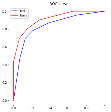
ROC

import matplotlib.pyplot as plt

y_test_proba_predict = model.predict_proba(X_test)[:,0]
y_train_proba_predict = model.predict_proba(X_train)[:,0]
fpr_test, tpr_test, th_test = metrics.roc_curve(y_test==0, y_test_proba_predict)
fpr_train, tpr_train, th_train = metrics.roc_curve(y_train==0, y_train_proba_predict)
plt.figure(figsize=[6,6])
plt.plot(fpr_test, tpr_test, color='blue',label='test')
plt.plot(fpr_train, tpr_train, color='red',label='train')
plt.legend()
plt.title('ROC curve')

AUC

metrics.roc_auc_score(y_true, y_predict_proba)

metrics.roc_auc_score(y_train==0, y_train_proba_predict), metrics.roc_auc_score(y_test==0, y_test_proba_predict)

回归模型的评价指标

• 误差绝对值的平均值 metrics.mean_absolute_error(y_true,y_pred)
• 误差平方的绝对值（MSE） metrics.mean_squared_error(y_true,y_pred)

综合评价指标（图）

• 验证曲线 validation_curve,参数不同时，各个评价指标的曲线
• 学习曲线 learning_curve, 数据集大小不同时，各个评价指标的曲线

对交易模型的评价

金融中的交易模型，几乎都属于上面说的对回归和分类模型。因此，对回归和分类模型的评价同样适用。下面具体分析，其内容基本没有超越上文

• 这个系统是不是黑盒 如果模型的内在逻辑很难用业务逻辑解释，那么要打上一个问号
• 系统与实际的相符程度
  • 测试数据是否覆盖一个经济周期
  • 佣金&滑点是否准确地考虑进去了
• 测试结果是否有统计意义
  • 交易次数越多，结果越可信
  • 系统盈利越分散，结果越可信。否则，盈利太集中，说明有可能运气成分居多
• 是否有过拟合
  • 参数越少越好。很多参数可能过拟合
  • 魔法数字：为何是20日移动平均？为何不是30日或21日？
  • 规则越简单，越不容易过拟合
  • 对参数的敏感程度（不要参数稍小变动导致交易效果巨量变动）

参考文献

王小川授课内容

Wikipedia