【logistics】理论与实现

2017年05月07日

Author: Guofei

文章归类: 2-1-有监督学习，文章编号: 220

版权声明：本文作者是郭飞。转载随意，但需要标明原文链接，并通知本人
原文链接：https://www.guofei.site/2017/05/07/LogisticRegression.html

Edit

logistics regression是一种典型的分类模型

logistic regression, logit regression, logit model这三个模型本质和用法非常相似，因此这里不加区分

logistic distribution

定义

CDF满足这个的随机变量叫做logistic distribution
F(x;μ,s)=11+e−(x−μ)/sF(x;μ,s)=11+e−(x−μ)/s

性质

不难推导出PDF：
f(x;μ,s)=e−(x−μ)/ss(1+e−(x−μ)/s)2f(x;μ,s)=e−(x−μ)/ss(1+e−(x−μ)/s)2

logistic regression

模型

P(Y=1∣x)=exp(wx)1+exp(wx)P(Y=1∣x)=exp⁡(wx)1+exp⁡(wx)

P(Y=0∣x)=11+exp(wx)P(Y=0∣x)=11+exp⁡(wx)

求参数的方法，就是经典的 MLE (极大似然估计)方法。
先求似然函数，
l(w;x)=∏i=1N[P(Y=1|x)]yi[P(Y=0|x)]1−yil(w;x)=∏i=1N[P(Y=1|x)]yi[P(Y=0|x)]1−yi
取对数后求argmaxlnl(w)argmaxln⁡l(w)
这是一个 凸函数 ，（凸函数的知识参见我的另一篇博文最优化方法理论篇）
由于是一个凸函数，可以用导数值为0确定最大值点，还可以用梯度下降法迭代求解最大值点。

推导似然函数：
令L(w;x)=lnl(w;x)L(w;x)=ln⁡l(w;x)L(w;x)=∑i=1N(yiwxi−ln(1+ewxi))L(w;x)=∑i=1N(yiwxi−ln⁡(1+ewxi))

w和x都是向量。下面研究向量的第j个分量
偏导数为：

∂L(w;x)∂wj=∑i=1N(yixij−ewxixij1+ewxi)=∑i=1N(yi−ewxi1+ewxi)xij∂L(w;x)∂wj=∑i=1N(yixij−ewxixij1+ewxi)=∑i=1N(yi−ewxi1+ewxi)xij

令导数为0，遗憾的是无法求出解析解。
因此用梯度法可以求解

Python实现（自己编程）

梯度法

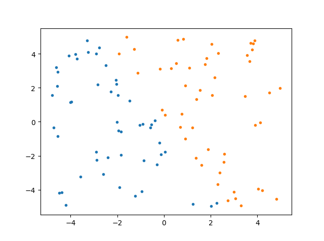
首先生成模拟数据

import numpy as np
import pandas as pd
import matplotlib.pyplot as plt
data = np.random.uniform(low=-5, high=5, size=(100, 2))
data=pd.DataFrame(data)
mask = (data.iloc[:, 0] + 0.5* data.iloc[:, 1])<0
data['y']=mask*1

data1 = data[data.iloc[:, 2] == 1] #为了画图，两类不同颜色
data2 = data[data.iloc[:, 2] == 0]
plt.plot(data1.iloc[:, 0], data1.iloc[:, 1], '.')
plt.plot(data2.iloc[:, 0], data2.iloc[:, 1], '.')
plt.show()

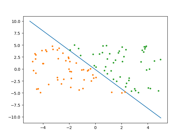
迭代求解：

alpha = 0.001 # 步长
step = 500   # 总共的迭代次数
m, n = data.shape
weights = np.ones((n, 1))

data_x = np.concatenate((np.ones((m, 1)), np.array(data.iloc[:, :2])), axis=1)  # 去掉y列，并添加全1的第一列
target = np.array(data.iloc[:, 2])
target.shape = -1, 1


def logistic(wTx):
    return 1 / (1 + np.exp(-wTx))


for i in range(step):
    wTx = np.dot(data_x, weights)
    output = logistic(wTx)
    errors = target - output
    weights = weights + alpha * np.dot(data_x.T, errors)

X = np.linspace(-5, 5, 100)
Y = -(weights[0] + X * weights[1]) / weights[2]


plt.plot(X, Y)
plt.plot(data1.iloc[:, 0], data1.iloc[:, 1], '.')
plt.plot(data2.iloc[:, 0], data2.iloc[:, 1], '.')
plt.show()

随机梯度下降法

随机梯度下降法并没有引入新理论，解决的主要问题是步长alpha的问题。
alpha太大，容易越过极值点，导致震荡不收敛。
alpha太小，收敛速度会降低。
算法的伪代码是这样的：

for 第i次迭代
    for 第j次收取
        alpha=2/(1+i+j)+0.001
        从全部样本中随机抽取样本，梯度下降，步长为alpha

Python实现（sklearn）

step1:建立模型1

from sklearn.datasets import load_iris
dataset=load_iris()

from sklearn import linear_model
clf=linear_model.LogisticRegression()
clf.fit(dataset.data,dataset.target)

关于参数的选择，一定要看sklearn官网 2
step2：模型使用

clf.predict(dataset.data)#判断数据属于哪个类别
clf.predict_proba(dataset.data)#判断属于各个类别的概率
clf.score(dataset.data,dataset.target)#准确率


clf.coef_ #系数
clf.intercept_ #截距
clf.n_iter_ #迭代次数

备注

筛选+回归

用到sklearn中的两个模型

RandomizedLogisticRegression用来筛选变量
LogisticRegression用来做逻辑回归

step1:用RandomizedLogisticRegression筛选有效变量

from sklearn.linear_model import LogisticRegression as LR
from sklearn.linear_model import RandomizedLogisticRegression as RLR
rlr = RLR() #建立随机逻辑回归模型，用于筛选变量
rlr.fit(x, y) #训练模型
rlr.get_support() #获取特征筛选结果,是一个boll类型的array
rlr.scores_#各个特征的分数，是1darray
print('通过随机逻辑回归模型筛选特征结束。')
print('有效特征为：%s' % ','.join(x.columns[rlr.get_support()]))

step2：用LogisticRegression做逻辑回归

x_new = x[x.columns[rlr.get_support()]] #筛选好特征
lr = LR() #建立逻辑回归模型
lr.fit(x_new, y) #用筛选后的特征数据来训练模型
print('逻辑回归模型训练结束。')
print('模型的平均正确率为：%s' % lr.score(x_new, y)) #给出模型的平均正确率，本例为81.4%

参考文献

您的支持将鼓励我继续创作！

【logistics】理论与实现