Over the last decade, the landscape of machine learning software development has undergone significant changes. Many frameworks have come and gone, but most have relied heavily on leveraging Nvidia's CUDA and performed best on Nvidia GPUs. However, with the arrival of PyTorch 2.0 and OpenAI's Triton, Nvidia's dominant position in this field, mainly due to its software moat, is being disrupted.

This report will touch on topics such as why Google’s TensorFlow lost out to PyTorch, why Google hasn’t been able to capitalize publicly on its early leadership of AI, the major components of machine learning model training time, the memory capacity/bandwidth/cost wall, model optimization, why other AI hardware companies haven’t been able to make a dent in Nvidia’s dominance so far, why hardware will start to matter more, how Nvidia’s competitive advantage in CUDA is wiped away, and a major win one of Nvidia’s competitors has at a large cloud for training silicon.

The 1,000-foot summary is that the default software stack for machine learning models will no longer be Nvidia’s closed-source CUDA. The ball was in Nvidia’s court, and they let OpenAI and Meta take control of the software stack. That ecosystem built its own tools because of Nvidia’s failure with their proprietary tools, and now Nvidia’s moat will be permanently weakened.

TensorFlow vs. PyTorch

A handful of years ago, the framework ecosystem was quite fragmented, but TensorFlow was the frontrunner. Google looked poised to control the machine learning industry. They had a first movers’ advantage with the most commonly used framework, TensorFlow, and by designing/deploying the only successful AI application-specific accelerator, TPU.

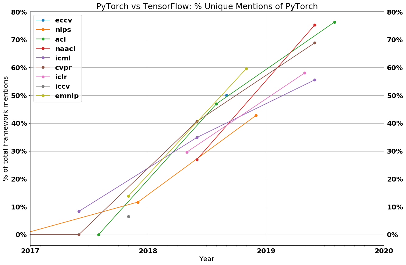
Instead, PyTorch won. Google failed to convert its first mover’s advantage into dominance of the nascent ML industry. Nowadays, Google is somewhat isolated within the machine learning community because of its lack of use of PyTorch and GPUs in favor of its own software stack and hardware. In typical Google fashion, they even have a 2nd framework called Jax that competes directly with TensorFlow.

There’s even endless talk of Google’s dominance in search and natural language processing waning due to large language models, particularly those from OpenAI and the various startups that utilize OpenAI APIs or are building similar foundational models. While we believe this doom and gloom is overblown, that story is for another day. Despite these challenges, Google is still at the forefront of the most advanced machine learning models. They invented transformers and remain state-of-the-art in many areas (PaLM, LaMBDA, Chinchilla, MUM, TPU).

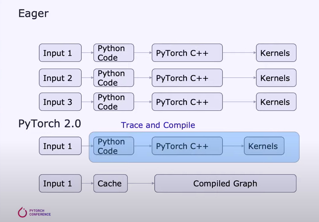
Back to why PyTorch won. While there was an element of wrestling control away from Google, it was primarily due to its increased flexibility and usability of PyTorch versus TensorFlow. If we boil it down to a first principal level, PyTorch differed from TensorFlow in using “Eager mode” rather than "Graph Mode."

Eager mode can be thought of as a standard scripting execution method. The deep learning framework executes each operation immediately, as it is called, line by line, like any other piece of Python code. This makes debugging and understanding your code more accessible, as you can see the results of intermediate operations and see how your model behaves.

In contrast, graph mode has two phases. The first phase is the definition of a computation graph representing the operations to perform. A computation graph is a series of interconnected nodes representing operations or variables, and the edges between nodes represent the data flow between them. The second phase is the deferred execution of an optimized version of the computation graph.

This two-phase approach makes it more challenging to understand and debug your code, as you cannot see what is happening until the end of the graph execution. This is analogous to "interpreted" vs. "compiled" languages, like python vs. C++. It's easier to debug Python, largely since it's interpreted.

While TensorFlow now has Eager mode by default, the research community and most large tech firms have settled around PyTorch. For a deeper explanation of why PyTorch won, see here.

Machine Learning Training Components

If we boil machine learning model training to its most simplistic form, there are two major time components in a machine learning model’s training time.

1. Compute (FLOPS):  Running dense matrix multiplication within each layer

2. Memory (Bandwidth): Waiting for data or layer weights to get to the compute resources. Common examples of bandwidth-constrained operations are various normalizations, pointwise operations, SoftMax, and ReLU.

In the past, the dominant factor in machine learning training time was compute time, waiting for matrix multiplies. As Nvidia’s GPUs continued to develop, this quickly faded away from being the primary concern.

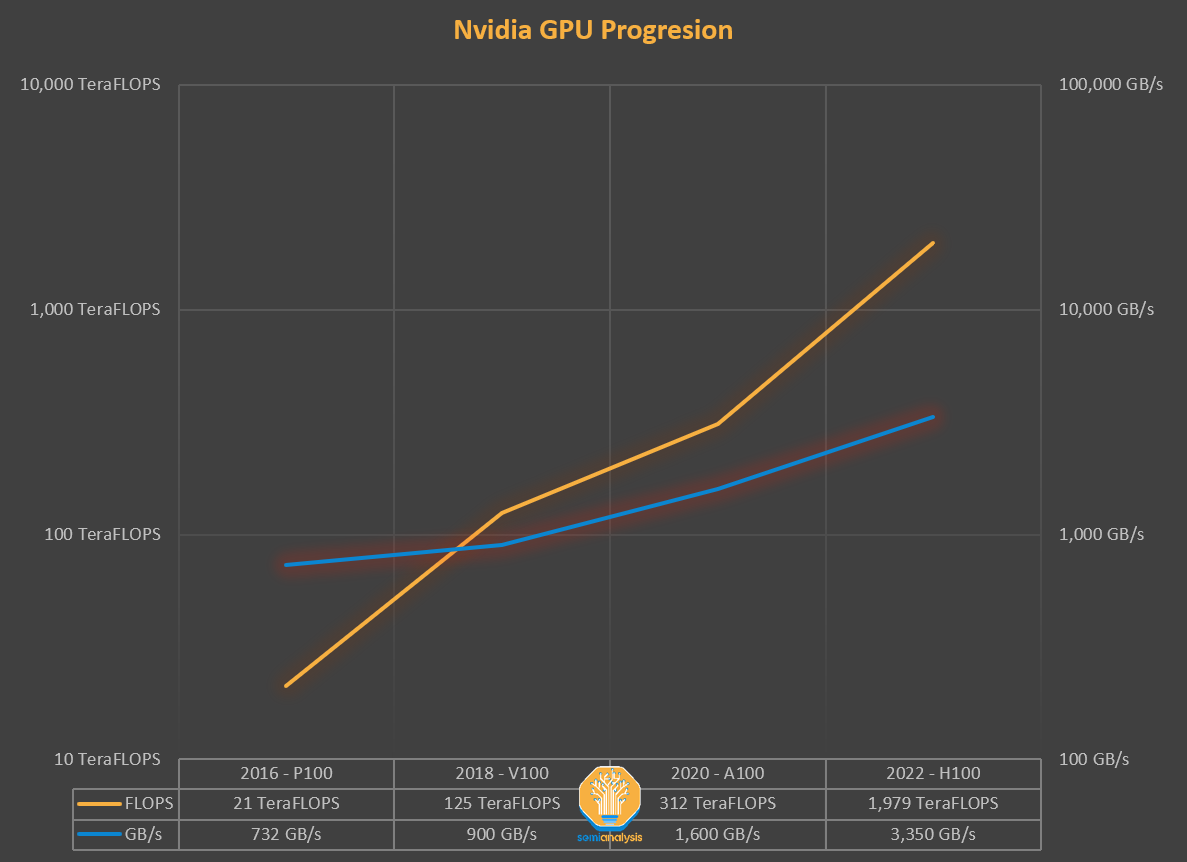
Nvidia’s FLOPS have increased multiple orders of magnitude by leveraging Moore’s Law, but primarily architectural changes such as the tensor core and lower precision floating point formats. In contrast, memory has not followed the same path.

If we go back to 2018, when the BERT model was state of the art, and the Nvidia V100 was the most advanced GPU, we could see that matrix multiplication was no longer the primary factor for improving a model’s performance. Since then, the most advanced models have grown 3 to 4 orders of magnitude in parameter count, and the fastest GPUs have grown an order of magnitude in FLOPS.

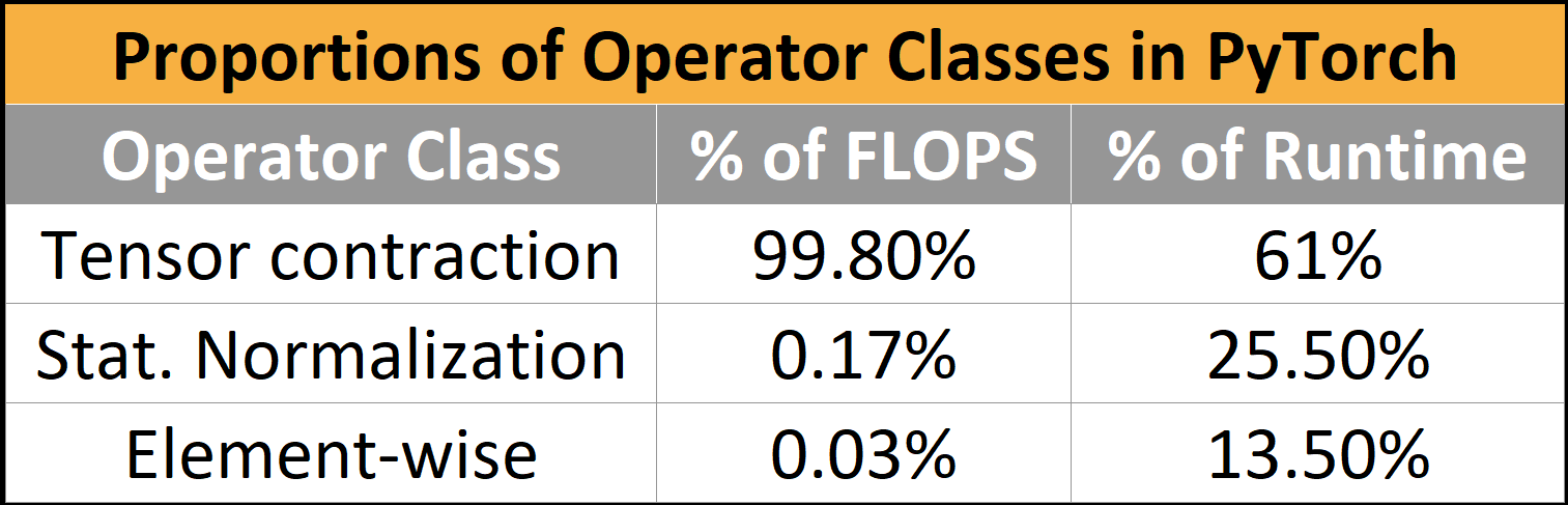
Even in 2018, purely compute-bound workloads made up 99.8% of FLOPS but only 61% of the runtime. The normalization and pointwise ops achieve 250x less FLOPS and 700x less FLOPS than matrix multiplications, respectively, yet they consume nearly 40% of the model’s runtime.

The Memory Wall

As models continue to soar in size, large language models take 100s gigabytes, if not terabytes, for the model weights alone. Production recommendation networks deployed by Baidu and Meta require dozens of terabytes of memory for their massive embedding tables. A huge chunk of the time in large model training/inference is not spent computing matrix multiplies, but rather waiting for data to get to the compute resources. The obvious question is why don’t architects put more memory closer to the compute. The answer is $$$.

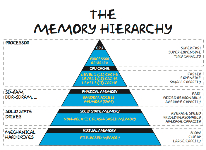
Memory follows a hierarchy from close and fast to slow and cheap. The nearest shared memory pool is on the same chip and is generally made of SRAM. Some machine-learning ASICs attempt to utilize huge pools of SRAM to hold model weights, but there are issues with this approach. Even Cerebras’ ~$5,000,000 wafer scale chips only have 40GB of SRAM on the chip. There isn’t enough memory capacity to hold the weights of a 100B+ parameter model.

Nvidia’s architecture has always used a much smaller amount of memory on the die. The current generation A100 has 40MB, and the next generation H100 has 50MB. 1GB of SRAM and the associated control logic/fabric on TSMC’s 5nm process node would require ~200mm^2 of silicon, or about 25% of the total logic area of an Nvidia datacenter GPU. Given that an A100 GPU costs $10k+ and the H100 is more like $20k+, economically, this is infeasible. Even when you ignore Nvidia’s ~75% gross margin on datacenter GPUs (~4x markup), the cost per GB of SRAM memory would still be in the $100s for a fully yielded product.

Furthermore, the cost of on-chip SRAM memory will not decrease much through conventional Moore’s Law process technology shrinks. The same 1GB of memory actually costs more with the next-generation TSMC 3nm process technology. While 3D SRAM will help with SRAM costs to some degree, that is only a temporary bend of the curve.

The next step down in the memory hierarchy is tightly coupled off-chip memory, DRAM. DRAM has an order magnitude higher latency than SRAM (~>100 nanoseconds vs. ~10 nanoseconds), but it’s also much cheaper ($1s a GB vs. $100s GB.)

DRAM followed the path of Moore’s Law for many decades. When Gordon Moore coined the term, Intel’s primary business was DRAM. His economic prediction about density and cost of transistors generally held true until ~2009 for DRAM. Since ~2012 though, the cost of DRAM has barely improved.

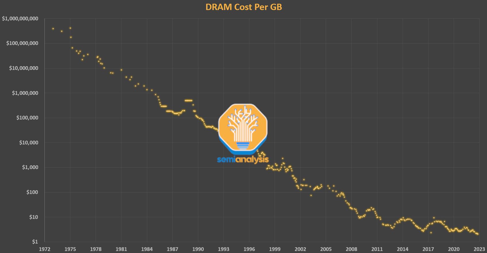
The demands for memory have only increased. DRAM now comprises 50% of the total server’s cost. This is the memory wall, and it has shown up in products. Comparing Nvidia’s 2016 P100 GPU to their 2022 H100 GPU that is just starting to ship, there is a 5x increase in memory capacity (16GB -> 80GB) but a 46x increase in FP16 performance (21.2 TFLOPS -> 989.5 TFLOPS).

While capacity is a significant bottleneck, it is intimately tied to the other major bottleneck, bandwidth. Increased memory bandwidth is generally obtained through parallelism. While standard DRAM is only a few dollars per GB today, to get the massive bandwidth machine learning requires, Nvidia uses HBM memory, a device comprised of 3D stacked layers of DRAM that requires more expensive packaging. HBM is in the $10 to $20 a GB range, including packaging and yield costs.

The cost constraints of memory bandwidth and capacity show up in Nvidia’s A100 GPUs constantly. The A100 tends to have very low FLOPS utilization without heavy optimization. FLOPS utilization measures the total computed FLOPS required to train a model vs. the theoretical FLOPS the GPUs could compute in a model’s training time.

Even with heavy optimizations from leading researchers, 60% FLOPS utilization is considered a very high utilization rate for large language model training. The rest of the time is overhead, idle time spent waiting for data from another calculation/memory, or recomputing results just in time to reduce memory bottlenecks.

From the current generation A100 to the next generation H100, the FLOPS grow by more than 6X, but memory bandwidth only grows by 1.65x. This has led to many fears of low utilization for H100. The A100 required many tricks to get around the memory wall, and more will need to be implemented with the H100.

The H100 brings distributed shared memory and L2 multicast to Hopper. The idea is that different SMs (think cores) can write directly to another SM’s SRAM (shared memory/L1 Cache). This effectively increases the size of the cache and reduces the required bandwidth of DRAM read/writes. Future architectures will rely on sending fewer operations to memory to minimize the impact of the memory wall. It should be noted that larger models tend to achieve higher utilization rates as FLOPS demands scale at 2^n, whereas memory bandwidth and capacity demands tend to scale at 2*n.

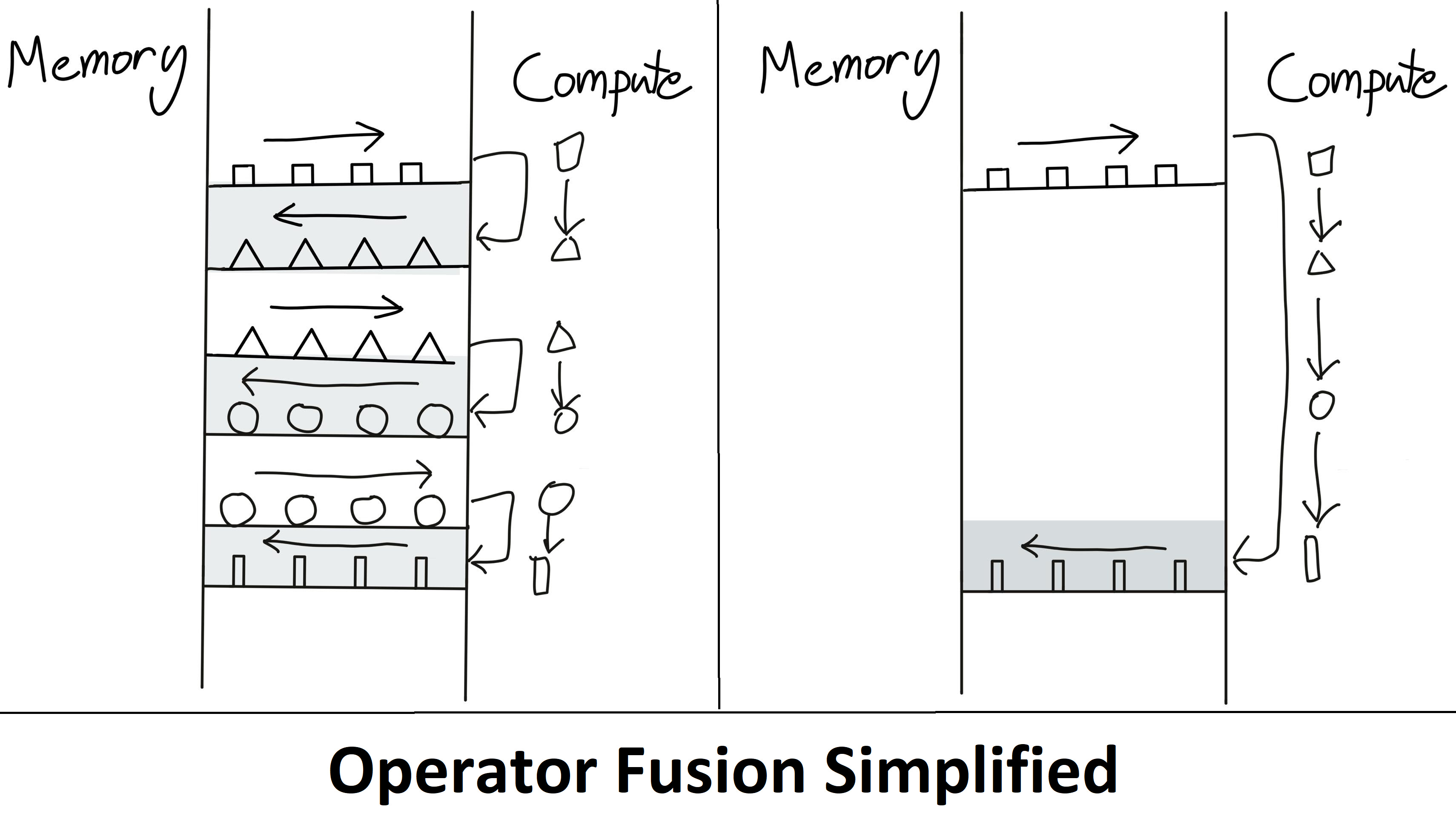
Operator Fusion – The Workaround

Just like with training ML models, knowing what regime you're in allows you to narrow in on optimizations that matters. For example, if you're spending all of your time doing memory transfers (i.e. you are in a memory-bandwidth bound regime), then increasing the FLOPS of your GPU won't help. On the other hand, if you're spending all of your time performing big chonky matmuls (i.e. a compute-bound regime), then rewriting your model logic into C++ to reduce overhead won't help.

https://horace.io/brrr_intro.html

Referring back to why PyTorch won, it was the increased flexibility and usability due to Eager mode, but moving to Eager mode isn’t all sunshine and rainbows. When executing in Eager mode, each operation is read from memory, computed, then sent to memory before the next operation is handled. This significantly increases the memory bandwidth demands if heavy optimizations aren’t done.

As such, one of the principal optimization methods for a model executed in Eager mode is called operator fusion. Instead of writing each intermediate result to memory, operations are fused, so multiple functions are computed in one pass to minimize memory reads/writes. Operator fusion improves operator dispatch, memory bandwidth, and memory size costs.

This optimization often involves writing custom CUDA kernels, but that is much more difficult than using simple python scripts. As a built-in compromise, PyTorch steadily implemented more and more operators over time natively within PyTorch. Many of these operators were simply multiple commonly used operations fused into a single, more complex function.

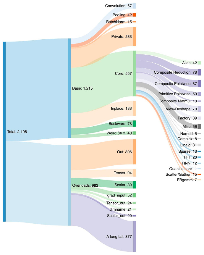
The increase in operators made both creating the model within PyTorch easier and the performance of Eager mode faster due to having fewer memory read/writes. The downside was that PyTorch ballooned to over 2,000 operators over a few years.

We would say software developers are lazy, but let’s be honest, almost all people are lazy. If they get used to one of the new operators within PyTorch, they will continue to use that. The developer may not even recognize the performance improvement but instead, use that operator because it means writing less code.

Additionally, not all operations can be fused. A significant amount of time is often spent deciding which operations to fuse and which operations to assign to specific compute resources at the chip and cluster levels. The strategy of which operations to fuse where, although generally similar, does vary significantly depending on the architecture.

Nvidia Is King

The growth in operators and position as the default has helped Nvidia as each operator was quickly optimized for their architecture but not for any other hardware. If an AI hardware startup wanted to fully implement PyTorch, that meant supporting the growing list of 2,000 operators natively with high performance.

The talent level required to train a massive model with high FLOPS utilization on a GPU grows increasingly higher because of all the tricks needed to extract maximum performance. Eager mode execution plus operator fusion means that software, techniques, and models that are developed are pushed to fit within the ratios of compute and memory that the current generation GPU has.

Everyone developing machine learning chips is beholden to the same memory wall. ASICs are beholden to supporting the most commonly used frameworks. ASICs are beholden to the default development methodology, GPU-optimized PyTorch code with a mix of Nvidia and external libraries. An architecture that eschews a GPU’s various non-compute baggage in favor of more FLOPS and a stiffer programming model makes very little sense in this context.

Ease of use is king.

The only way to break the vicious cycle is for the software that runs models on Nvidia GPUs to transfer seamlessly to other hardware with as little effort as possible. As model architectures stabilize and abstractions from PyTorch 2.0, OpenAI Triton, and MLOps firms such as MosaicML become the default, the architecture and economics of the chip solution starts to become the biggest driver of the purchase rather than the ease of use afforded to it by Nvidia’s superior software.

PyTorch 2.0

The PyTorch Foundation was established and moved out from under the wings of Meta just a few months ago. Alongside this change to an open development and governance model, 2.0 has been released for early testing with full availability in March. PyTorch 2.0 brings many changes, but the primary difference is that it adds a compiled solution that supports a graph execution model. This shift will make properly utilizing various hardware resources much easier.

PyTorch 2.0 brings an 86% performance improvement for training on Nvidia’s A100 and 26% on CPUs for inference! This dramatically reduces the compute time and cost required for training a model. These benefits could extend to other GPUs and accelerators from AMD, Intel, Tenstorrent, Luminous Computing, Tesla, Google, Amazon, Microsoft, Marvell, Meta, Graphcore, Cerebras, SambaNova, etc.

The performance improvements from PyTorch 2.0 will be larger for currently unoptimized hardware. Meta and other firms’ heavy contribution to PyTorch stems from the fact that they want to make it easier to achieve higher FLOPS utilization with less effort on their multi-billion-dollar training clusters made of GPUs. They are also motivated to make their software stacks more portable to other hardware to introduce competition to the machine learning space.

PyTorch 2.0 also brings advancements to distributed training with better API support for data parallelism, sharding, pipeline parallelism, and tensor parallelism. In addition, it supports dynamic shapes natively through the entire stack, which among many other examples, makes varying sequence lengths for LLMs much easier to support. This is the first time a major compiler supports Dynamic Shapes from training to inference.

PrimTorch

Writing a performant backend for PyTorch that fully supports all 2,000+ operators has been difficult for every machine learning ASIC except for Nvidia GPUs. PrimTorch brings the number of operators down to ~250 primitive operators while also keeping usability unchanged for end users of PyTorch. PrimTorch makes the implementation of different, non-Nvidia backends to PyTorch much simpler and more accessible. Custom hardware and system vendors can bring up their software stacks more easily.

TorchDynamo

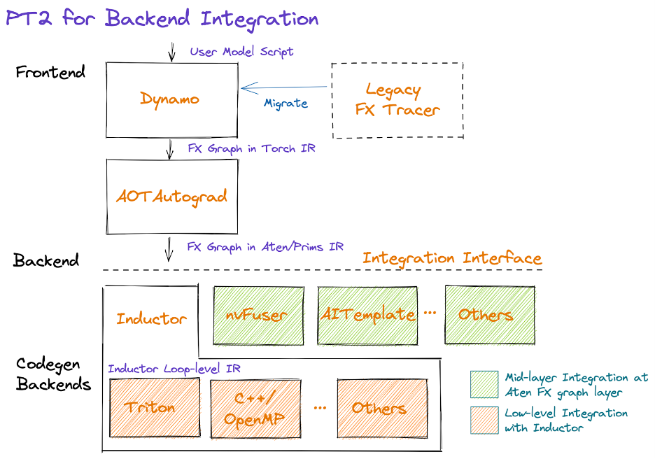
Moving to graph mode requires a robust graph definition. Meta and PyTorch have been attempting to work on implementing this for ~5 years, but every solution they came up with had significant drawbacks. They finally cracked the puzzle with TorchDynamo. TorchDynamo will ingest any PyTorch user script, including those that call outside 3rd party libraries, and generate an FX graph.

Dynamo lowers all complex operations to the ~250 primitive operations in PrimTorch. Once the graph is formed, unused operations are discarded, and the graph determines which intermediate operations need to be stored or written to memory and which can potentially be fused. This dramatically reduces the overhead within a model while also being seamless for the user.

TorchDynamo already works for over 99% of the 7,000 PyTorch models tested, including those from OpenAI, HuggingFace, Meta, Nvidia, Stability.AI, and more, without any changes to the original code. The 7,000 models tested were indiscriminately chosen from the most popular projects using PyTorch on GitHub.

Google’s TensorFlow/Jax and other graph mode execution pipelines generally require the user to ensure their model fits into the compiler architecture so that the graph can be captured. Dynamo changes this by enabling partial graph capture, guarded graph capture, and just-in-time recapture.

• Partial graph capture allows the model to include unsupported/non-python constructs. When a graph cannot be generated for that portion of the model, a graph break is inserted, and the unsupported constructs will be executed in eager mode between the partial graphs.

• Guarded graph capture checks if the captured graph is valid for execution. A guard is a change that would require recompilation. This is important because running the same code multiple times won't recompile multiple times.

• Just-in-time recapture allows the graph to be recaptured if the captured graph is invalid for execution.

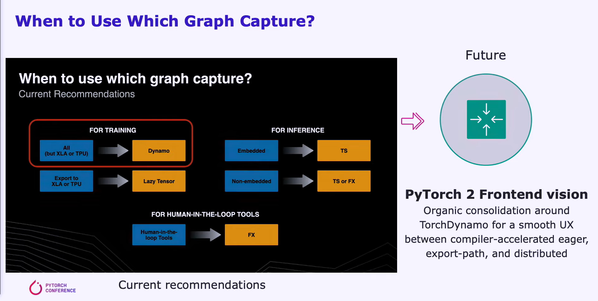
PyTorch’s goal is to create a unified front end with a smooth UX that leverages Dynamo to generate graphs. The user experience of this solution would be unchanged, but the performance can be significantly improved. Capturing the graph means execution can be parallelized more efficiently over a large base of compute resources.

Dynamo and AOT Autograd then pass the optimized FX graphs to the PyTorch native compiler level, TorchInductor. Hardware companies can also take this graph and input it into their own backend compilers.

TorchInductor

TorchInductor is a python native deep learning compiler that generates fast code for multiple accelerators and backends. Inductor will take the FX graphs, which have ~250 operators, and lowers them to ~50 operators. Inductor then moves to a scheduling phase where operators are fused, and memory planning is determined.

Inductor then goes to the “Wrapper Codegen,” which generates code that runs on the CPU, GPU, or other AI accelerators. The wrapper codegen replaces the interpreter part of a compiler stack and can call kernels and allocate memory. The backend code generation portion leverages OpenAI Triton for GPUs and outputs PTX code. For CPUs, an Intel compiler generates C++ (will work on non-Intel CPUs too).

More hardware will be supported going forward, but the key is that Inductor dramatically reduces the amount of work a compiler team must do when making a compiler for their AI hardware accelerator. Furthermore, the code is more optimized for performance. There are significant reductions in memory bandwidth and capacity requirements.

We didn't want to build a compiler that only supported GPUs. We wanted something that could scale to support a wide variety of hardware back ends, and having a C++ as well as [OpenAI] Triton forces that generality.

Jason Ansel – Meta AI

OpenAI Triton

OpenAI’s Triton is very disruptive angle to Nvidia’s closed-source software moat for machine learning. Triton takes in Python directly or feeds through the PyTorch Inductor stack. The latter will be the most common use case. Triton then converts the input to an LLVM intermediate representation and then generates code. In the case of Nvidia GPUs, it directly generates PTX code, skipping Nvidia’s closed-source CUDA libraries, such as cuBLAS, in favor of open-source libraries, such as cutlass.

CUDA is commonly used by those specializing in accelerated computing, but it is less well-known among machine learning researchers and data scientists. It can be challenging to use efficiently and requires a deep understanding of the hardware architecture, which can slow down the development process. As a result, machine learning experts may rely on CUDA experts to modify, optimize, and parallelize their code.

Triton bridges the gap enabling higher-level languages to achieve performance comparable to those using lower-level languages. The Triton kernels themselves are quite legible to the typical ML researcher which is huge for usability. Triton automates memory coalescing, shared memory management, and scheduling within SMs. Triton is not particularly helpful for the element-wise matrix multiplies, which are already done very efficiently. Triton is incredibly useful for costly pointwise operations and reducing overhead from more complex operations such as Flash Attention that involve matrix multiplies as a portion of a larger fused operation.

Share

OpenAI Triton only officially supports Nvidia GPUs today, but that is changing in the near future. Multiple other hardware vendors will be supported in the future, and this open-source project is gaining incredible steam. The ability for other hardware accelerators to integrate directly into the LLVM IR that is part of Triton dramatically reduces the time to build an AI compiler stack for a new piece of hardware.

Nvidia’s colossal software organization lacked the foresight to take their massive advantage in ML hardware and software and become the default compiler for machine learning. Their lack of focus on usability is what enabled outsiders at OpenAI and Meta to create a software stack that is portable to other hardware.

The rest of this report will point out the specific hardware accelerator that has a huge win at Microsoft, as well as multiple companies’ hardware that is quickly being integrated into the PyTorch 2.0/OpenAI Trion software stack. Furthermore, it will share the opposing view as a defense of Nvidia’s moat/strength in the AI training market.

Get 20% off a group subscription