New method identifies the root causes of statistical outliers

Amazon ICML paper proposes information-theoretic measurement of quantitative causal contribution.

Outliers are rare observations where a system deviates from its usual behavior. They arise in many real-world applications (e.g., medicine, finance) and present a greater demand for explanation than ordinary events. How can we identify the "root causes" of outliers once they are detected?

The problem of outliers is one of the oldest problems in statistics. It has been the subject of academic investigation for more than a century. Although a lot has been done on detecting outliers, a formal way to define the “root causes” of outliers has been lacking.

This week, at the International Conference on Machine Learning (ICML), we are presenting our work on identifying the root causes of outliers. Our first task was to introduce a formal definition of “root cause”, because we were not able to find one in the academic literature.

Our definition includes a formalization of the quantitative causal contribution of each of the root causes of an observed outlier. In other words, the contribution describes the degree to which a variable is responsible for the outlier event. This also relates to philosophical questions; even the purely qualitative question of whether an event is an “actual cause” of others is an ongoing debate among philosophers.

Our approach is based on graphical causal models, a formal framework developed by Turing Award winner Judea Pearl to model cause-effect relationships between variables in a system. It has two key ingredients. The first is a causal diagram, which visually represents the cause-effect relationships among observed variables, with arrows from the nodes representing causes to the nodes representing effects. The second is a set of causal mechanisms, which describe how the values of each node are generated from the values of its parents (i.e., direct causes) in the causal diagram.

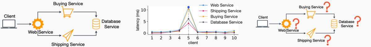
Imagine, for instance, a retail website powered by distributed web services. A customer experiences an unusually slow loading time. Why? Is it a slow database in the back end? A malfunctioning buying service?

At left, we have the dependencies between the distributed web services that power a simple hypothetical retail website. In the middle, a customer (with ID 5) experiences a very slow loading time. Our goal is to identify its root causes among the distributed services (right).

There exist many outlier detection algorithms. To identify the root causes of outliers detected by one of these algorithms, we first introduce an information-theoretic (IT) outlier score, which probabilistically calibrates existing outlier scores.

Our outlier score relies on the notion of the tail probability — the probability that a random variable exceeds a threshold value. The IT outlier score of an event is the negative logarithm of the event’s tail probability under some transformation. It is inspired by Claude Shannon’s definition of the information content of a random event in information theory.

The lower the likelihood of observing events more extreme than the event in question, the more information that event carries, and the larger its IT outlier score. Probabilistic calibration also renders IT outlier scores comparable across variables with different dimension, range, and scaling.

Counterfactuals

To attribute the outlier event to a variable, we ask the counterfactual question “Would the event not have been an outlier had the causal mechanism of that variable been normal?” The counterfactuals are the third rung on Pearl’s ladder of causation and hence require functional causal models (FCMs) as the causal mechanisms of variables.

In an FCM, each variable Xj is a function of its observed parents PAj (with direct arrows to Xj) in the causal diagram and an unobserved noise variable Nj. As root nodes — those without observed parents — have only noise variables, the joint distribution of noise variables gives rise to the stochastic properties of observed variables.

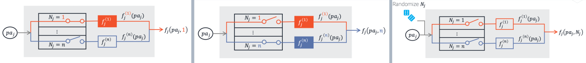
The unobserved noise variables play a special role: we can think of Nj as a random switch that selects a deterministic function (or mechanism) from a set of functions Fj defined from direct causes PAj to their effect Xj. If, instead of fixing the value of the noise term Nj, we set it to random values drawn from some distribution, then the functions from the set Fjare also selected at random, and we can use this procedure to assign normal deterministic mechanisms to Xj.

Although this randomization operation might seem infeasible if we think of the noise variable as something not under our control — and even worse, not even observable — we can interpret it as an intervention on the observed variable.

On the left, for the observed pair (xj, paj) of variable Xj and its parents PAj, the deterministic mechanism fj(1) of variable Xj is identified by the noise value (Nj = 1) corresponding to the pair (xj, paj). In the middle, a different value of noise (Nj = n) identifies a counterfactual deterministic mechanism fj(n). On the right, by drawing random samples of the noise term Nj according to some distribution, we assign “normal” deterministic mechanisms to Xj.

To attribute the outlier event xn of target variable Xn to a variable Xj, we first replace the deterministic mechanism of Xjby normal causal mechanisms (the orange background indicates the replacement). Then we measure the impact of this replacement on the log tail probability of the outlier event.

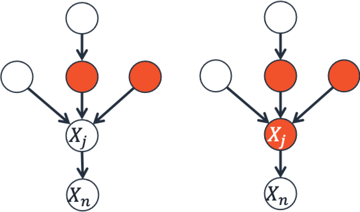
To attribute the outlier event xn (of target variable Xn) to a variable Xj, we first replace the deterministic mechanism corresponding to its observation xj by normal mechanisms. The impact of this replacement on the log tail probability defines the contribution of Xj to the outlier event. In particular, the contribution measures the factor by which replacing the causal mechanism of Xj with normal mechanisms (by drawing random samples of the noise Nj) decreases the likelihood of the outlier event. But the contribution computed this way depends on the order in which we replace the causal mechanisms. This dependence on ordering introduces arbitrariness into the attribution procedure.

To get rid of the dependence on the ordering of variables, we take the average contribution over all orderings, which is also the idea behind the Shapley value approach in game theory. The Shapley contributions sum up to the IT outlier score of the outlier event.

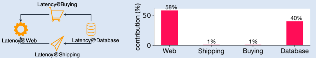
To get a high-level idea of how our approach works, consider again the retail-website example mentioned above. Dependencies between web services are typically available as a dependency graph. By inverting the arrows in the dependency graph, we obtain the causal graph of latencies of services. From training samples of observed latencies, we learn the causal mechanisms. The causal mechanisms may also be established directly using subject matter expertise. Our approach uses those to attribute the slow loading time for the specific client to its most likely root causes among the web services.

On the left, we have the causal graph of latencies of services, which is obtained by inverting the arrows of the dependency graph of services. By learning the causal mechanisms of nodes from training data, our approach yields the contributions of each node to the outlier event — here, the unusually high latency of the web service. As the Shapley contributions sum up to the IT outlier score of the outlier event, we are able to show the relative contribution of ancestors — here, the services.

If you would like to apply our approach to your use case, the implementation is available in the “gcm” package in the Python DoWhy library. To get started quickly, you can check out our example notebook.