

二值图像的连通域标记
source link: https://zhajiman.github.io/post/connected_component_labelling/
Go to the source link to view the article. You can view the picture content, updated content and better typesetting reading experience. If the link is broken, please click the button below to view the snapshot at that time.

连通域标记(connected component labelling)即找出二值图像中互相独立的各个连通域并加以标记,如下图所示(引自 MarcWang 的 Gist)
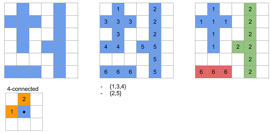
可以看到图中有三个独立的区域,我们希望找到并用数字标记它们,以便计算各个区域的轮廓、外接形状、质心等参数。连通域标记最基本的两个算法是 Seed-Filling 算法和 Two-Pass 算法,下面便来分别介绍它们,并用 Python 加以实现。
(2022-01-04 更新:修复了 seed_filling 重复追加相邻像素的问题,修改了其它代码的表述。)
Seed-Filling 算法
直译即种子填充,以图像中的特征像素为种子,然后不断向其它连通区域蔓延,直至将一个连通域完全填满。示意动图如下(引自 icvpr 的博客)

具体思路为:循环遍历图像中的每一个像素,如果某个像素是未被标记过的特征像素,那么用数字对其进行标记,并寻找与之相邻的未被标记过的特征像素,再对这些像素也进行标记,然后以同样的方法继续寻找与这些像素相邻的像素并加以标记……如此循环往复,直至将这些互相连通的特征像素都标记完毕,此即连通域 1。接着继续遍历图像像素,看能不能找到下一个连通域。下面的实现采用深度优先搜索(DFS)的策略:将与当前位置相邻的特征像素压入栈中,弹出栈顶的像素,再把与这个像素相邻的特征像素压入栈中,重复操作直至栈内像素清空。
import numpy as np

def seed_filling(image, diag=False):
    '''
    用Seed-Filling算法标记图片中的连通域.

    Parameters
    ----------
    image : ndarray, shape (nrow, ncol)
        图片数组,零值表示背景,非零值表示特征.

    diag : bool
        指定邻域是否包含四个对角.

    Returns
    -------
    labelled : ndarray, shape (nrow, ncol), dtype int
        表示连通域标签的数组,0表示背景,从1开始表示标签.

    nlabel : int
        连通域的个数.
    '''
    # 用-1表示未被标记过的特征像素.
    image = np.asarray(image, dtype=bool)
    nrow, ncol = image.shape
    labelled = np.where(image, -1, 0)

    # 指定邻域的范围.
    if diag:
        offsets = [
            (-1, -1), (-1, 0), (-1, 1),(0, -1),
            (0, 1), (1, -1), (1, 0), (1, 1)
        ]
    else:
        offsets = [(-1, 0), (0, -1), (0, 1), (1, 0)]

    def get_neighbor_indices(row, col):
        '''获取(row, col)位置邻域的下标.'''
        for (dx, dy) in offsets:
            x = row + dx
            y = col + dy
            if 0 <= x < nrow and 0 <= y < ncol:
                yield x, y

    label = 1
    for row in range(nrow):
        for col in range(ncol):
            # 跳过背景像素和已经标记过的特征像素.
            if labelled[row, col] != -1:
                continue
            # 标记当前位置和邻域内的特征像素.
            current_indices = []
            labelled[row, col] = label
            for neighbor_index in get_neighbor_indices(row, col):
                if labelled[neighbor_index] == -1:
                    labelled[neighbor_index] = label
                    current_indices.append(neighbor_index)
            # 不断寻找与特征像素相邻的特征像素并加以标记,直至再找不到特征像素.
            while current_indices:
                current_index = current_indices.pop()
                labelled[current_index] = label
                for neighbor_index in get_neighbor_indices(*current_index):
                    if labelled[neighbor_index] == -1:
                        labelled[neighbor_index] = label
                        current_indices.append(neighbor_index)
            label += 1

    return labelled, label - 1
Two-Pass 算法
顾名思义,是会对图像过两遍循环的算法。第一遍循环先粗略地对特征像素进行标记,第二遍循环中再根据不同标签之间的关系对第一遍的结果进行修正。示意动图如下(引自 icvpr 的博客)

具体思路为
- 第一遍循环时,若一个特征像素周围全是背景像素,那它很可能是一个新的连通域,需要赋予其一个新标签。如果这个特征像素周围有其它特征像素,则说明它们之间互相连通,此时随便用它们中的一个旧标签值来标记当前像素即可,同时要用并查集记录这些像素的标签间的关系。
- 因为我们总是只利用了当前像素邻域的信息(考虑到循环方向是从左上到右下,邻域只需要包含当前像素的上一行和本行的左边),所以第一遍循环中找出的那些连通域可能会在邻域之外相连,导致同一个连通域内的像素含有不同的标签值。不过利用第一遍循环时获得的标签之间的关系(记录在并查集中),可以在第二遍循环中将同属一个集合(连通域)的不同标签修正为同一个标签。
- 经过第二遍循环的修正后,虽然假独立区域会被归并,但它所持有的标签值依旧存在,这就导致本应连续的标签值序列中有缺口(gap)。所以依据需求可以进行第三遍循环,去掉这些缺口,将标签值修正为连续的整数序列。
其中提到的并查集是一种处理不相交集合的数据结构,支持查询元素所属、合并两个集合的操作。利用它就能处理标签和连通域之间的从属关系。我是看 算法学习笔记(1) : 并查集 这篇知乎专栏学的。下面的实现中仅采用路径压缩的优化,合并两个元素时始终让大的根节点被合并到小的根节点上,以保证连通域标签值的排列顺序跟数组的循环方向一致。
from scipy.stats import rankdata

class UnionFind:
    '''用列表实现简单的并查集.'''
    def __init__(self, n):
        '''创建含有n个节点的并查集,每个元素指向自己.'''
        self.parents = list(range(n))

    def find(self, i):
        '''递归查找第i个节点的根节点,同时压缩路径.'''
        parent = self.parents[i]
        if parent == i:
            return i
        else:
            root = self.find(parent)
            self.parents[i] = root
            return root

    def union(self, i, j):
        '''合并节点i和j所属的两个集合.保证大的根节点被合并到小的根节点上.'''
        root_i = self.find(i)
        root_j = self.find(j)
        if root_i < root_j:
            self.parents[root_j] = root_i
        elif root_i > root_j:
            self.parents[root_i] = root_j
        else:
            return None

def two_pass(image, diag=False):
    '''
    用Two-Pass算法标记图片中的连通域.

    Parameters
    ----------
    image : ndarray, shape (nrow, ncol)
        图片数组,零值表示背景,非零值表示特征.

    diag : bool
        指定邻域是否包含四个对角.

    Returns
    -------
    labelled : ndarray, shape (nrow, ncol), dtype int
        表示连通域标签的数组,0表示背景,从1开始表示标签.

    nlabel : int
        连通域的个数.
    '''
    image = np.asarray(image, dtype=bool)
    nrow, ncol = image.shape
    labelled = np.zeros_like(image, dtype=int)
    uf = UnionFind(image.size // 2)

    # 指定邻域的范围,相比seed-filling只有半边.
    if diag:
        offsets = [(-1, -1), (-1, 0), (-1, 1), (0, -1)]
    else:
        offsets = [(-1, 0), (0, -1)]

    def get_neighbor_indices(row, col):
        '''获取(row, col)位置邻域的下标.'''
        for (dx, dy) in offsets:
            x = row + dx
            y = col + dy
            if 0 <= x < nrow and 0 <= y < ncol:
                yield x, y

    label = 1
    for row in range(nrow):
        for col in range(ncol):
            # 跳过背景像素.
            if not image[row, col]:
                continue
            # 寻找邻域内特征像素的标签.
            feature_labels = []
            for neighbor_index in get_neighbor_indices(row, col):
                neighbor_label = labelled[neighbor_index]
                if neighbor_label > 0:
                    feature_labels.append(neighbor_label)
            # 当前位置取邻域内的标签,同时记录邻域内标签间的关系.
            if feature_labels:
                first_label = feature_labels[0]
                labelled[row, col] = first_label
                for feature_label in feature_labels[1:]:
                    uf.union(first_label, feature_label)
            # 若邻域内没有特征像素,当前位置获得新标签.
            else:
                labelled[row, col] = label
                label += 1

    # 获取所有集合的根节点,由大小排名得到标签值.
    roots = [uf.find(i) for i in range(label)]
    labels = rankdata(roots, method='dense') - 1
    # 利用advanced indexing替代循环修正标签数组.
    labelled = labels[labelled]

    return labelled, labelled.max()
其中对标签值进行重新排名的部分用到了 scipy.stats.rankdata 函数,自己写循环来实现也可以,但当标签值较多时效率会远低于这个函数。从代码来看,Two-Pass 算法比 Seed-Filling 算法更复杂一些,但因为不需要进行递归式的填充,所以理论上要比后者更快。
许多图像处理的包里有现成的函数,例如
scipy.ndimage.labelskimage.measure.labelcv2.connectedComponets
具体信息和用法请查阅文档。顺便测一下各方法的速度,如下图所示(通过 IPython 的 %timeit 测得)
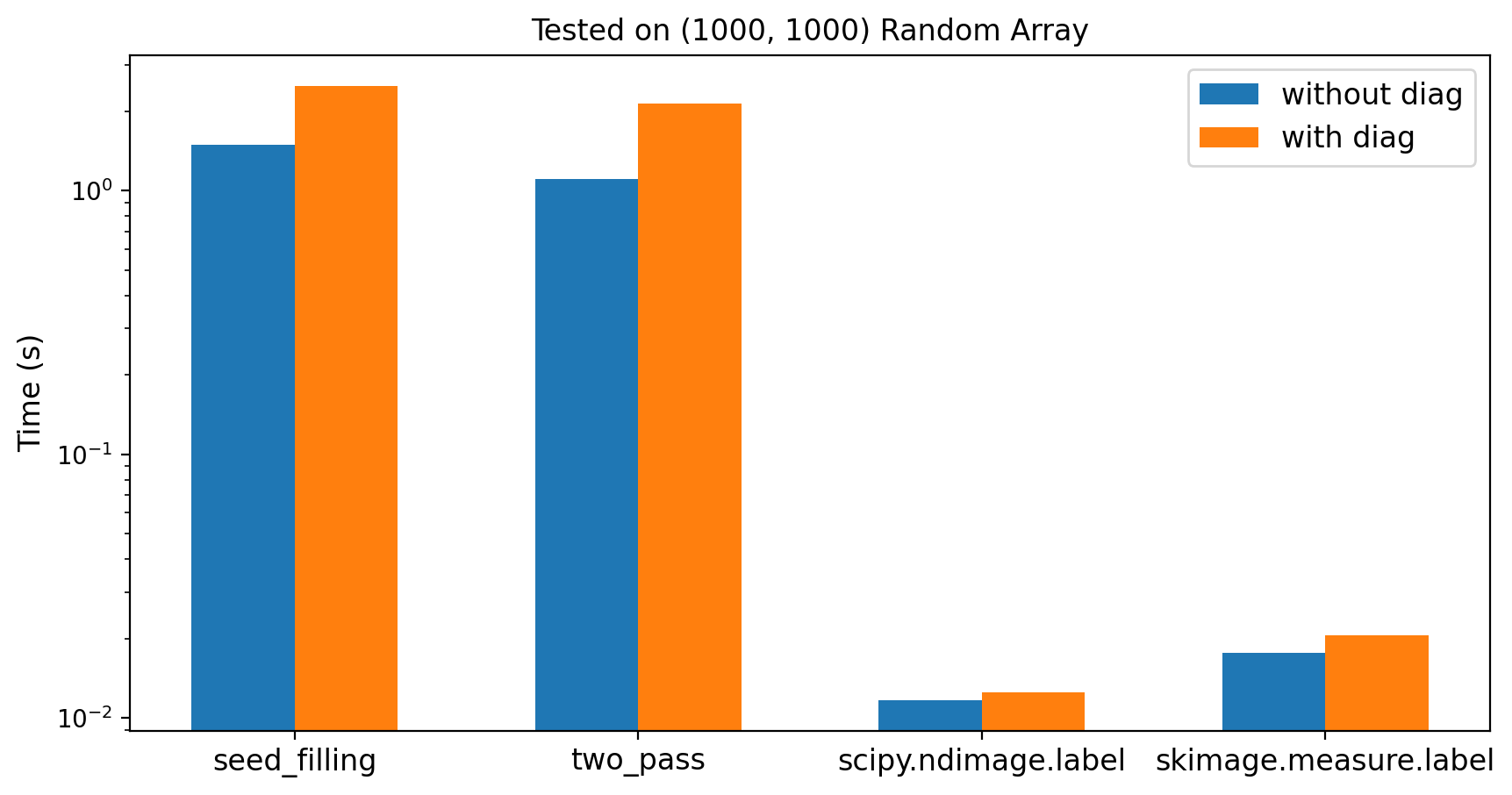
显然调包要比手工实现快 100 倍,这是因为 scipy.ndimage.label 和 skimage.measure.label 使用了更高级的算法和 Cython 代码。因为我不懂 OpenCV,所以这里没有展示 cv2.connectedComponets 的结果。
值得注意的是,虽然上一节说理论上 Two-Pass 算法比 Seed-Filling 快,但测试结果相差不大,这可能是由于纯 Python 实现体现不出二者的差异(毕竟完全没用到 NumPy 数组的向量性质),也可能是我代码写的太烂,还请懂行的读者指点一下。
以一个随机生成的 (50, 50) 的二值数组为例,展示 scipy.ndimage.label、seed_filling 和 two_pass 三者的效果,采用 8 邻域连通,如下图所示
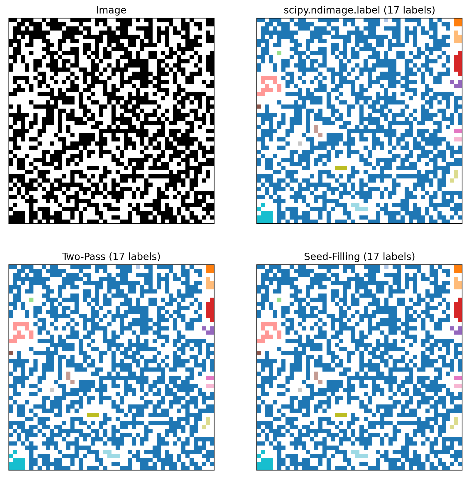
可以看到三种方法都找出了 17 个连通域,并且连标签顺序都一模一样(填色相同)。不过若 Two-Pass 法中的并查集采用其它合并策略,标签顺序就很可能发生变化。下面再以一个更复杂的 (800, 800) 大小的空露露图片为例
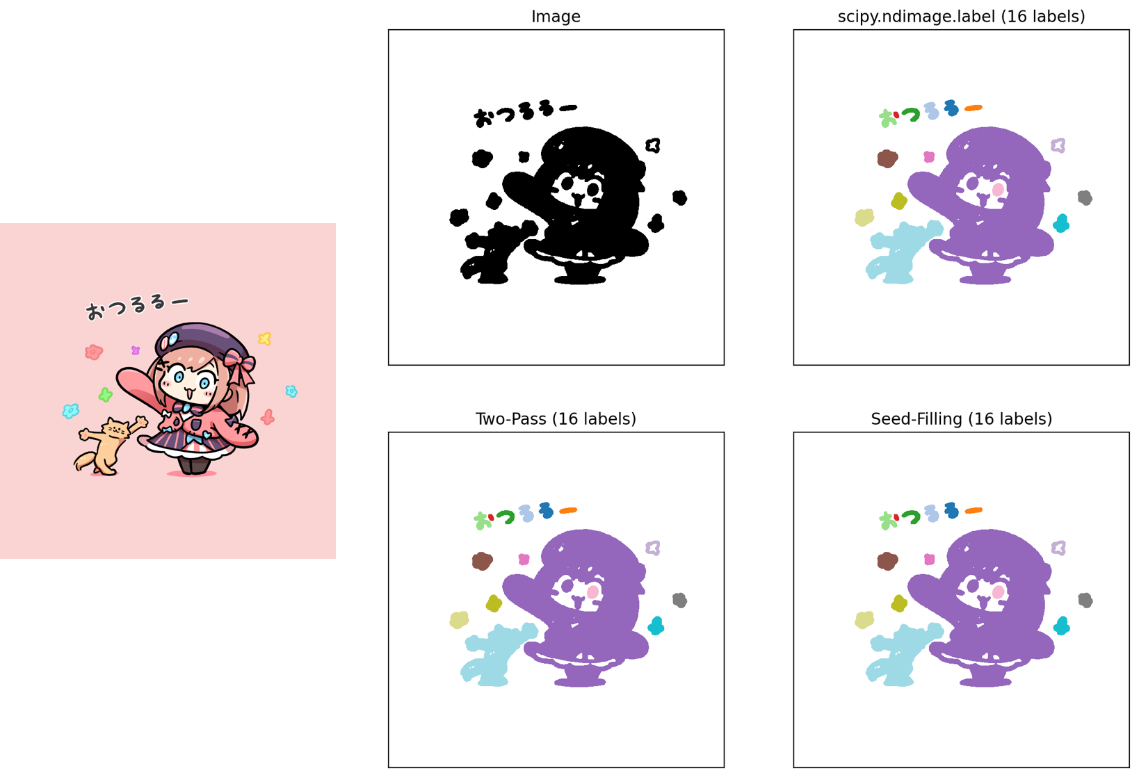
将图片二值化后再进行连通域标记,可以看到おつるる的字样被区分成多个区域,猫猫和露露也都被识别了出来。代码如下
import numpy as np
from PIL import Image
from scipy import ndimage
import matplotlib.pyplot as plt
import matplotlib.colors as mcolors

from connected_components import two_pass, seed_filling

if __name__ == '__main__':
    # 将测试图片二值化.
    picname = 'ruru.png'
    image = Image.open(picname)
    image = np.array(image.convert('L'))
    image = ndimage.gaussian_filter(image, sigma=2)
    image = np.where(image < 220, 1, 0)

    # 设置二值图像与分类图像所需的cmap.
    cmap1 = mcolors.ListedColormap(
        ['white', 'black'])
    white = np.array([1, 1, 1])
    cmap2 = mcolors.ListedColormap(
        np.vstack([white, plt.cm.tab20.colors])
    )

    fig, axes = plt.subplots(2, 2, figsize=(10, 10))

    # 关闭ticks的显示.
    for ax in axes.flat:
        ax.xaxis.set_visible(False)
        ax.yaxis.set_visible(False)

    # 显示二值化的图像.
    axes[0, 0].imshow(image, cmap=cmap1, interpolation='nearest')
    axes[0, 0].set_title('Image', fontsize='large')

    # 显示scipy.ndimage.label的结果.
    # 注意imshow中需要指定interpolation为'nearest'或'none',否则结果有紫边.
    s = np.ones((3, 3), dtype=int)
    labelled, nlabel = ndimage.label(image, structure=s)
    axes[0, 1].imshow(labelled, cmap=cmap2, interpolation='nearest')
    axes[0, 1].set_title(
        f'scipy.ndimage.label ({nlabel} labels)', fontsize='large'
    )

    # 显示Two-Pass算法的结果.
    labelled, nlabel = two_pass(image, diag=True)
    axes[1, 0].imshow(labelled, cmap=cmap2, interpolation='nearest')
    axes[1, 0].set_title(f'Two-Pass ({nlabel} labels)', fontsize='large')

    # 显示Seed-Filling算法的结果.
    labelled, nlabel = seed_filling(image, diag=True)
    axes[1, 1].imshow(labelled, cmap=cmap2, interpolation='nearest')
    axes[1, 1].set_title(f'Seed-Filling ({nlabel} labels)', fontsize='large')

    fig.savefig('image.png', dpi=200, bbox_inches='tight')
    plt.close(fig)
不只是邻接
虽然 scipy.ndimage.label 和 skimage.measure.label 要比手工实现更快,但它们都只支持 4 邻域和 8 邻域的连通规则,而手工实现还可以采用别的连通规则。例如,改动一下 seed_filling 中关于 offsets 的部分,使之能够表示以当前像素为原点,r 为半径的圆形邻域
offsets = []
for i in range(-r, r + 1):
    k = r - abs(i)
    for j in range(-k, k + 1):
        offsets.append((i, j))
offsets.remove((0, 0))  # 去掉原点.
在某些情况下也许能派上用场。
网上很多教程抄了这篇,但里面 Two-Pass 算法的代码里不知道为什么没用并查集,可能会有问题。
OpenCV_连通区域分析(Connected Component Analysis-Labeling)
一篇英文的对 Two-Pass 算法的介绍,Github 上还带有 Python 实现。
代码参考了
Recommend
About Joyk
Aggregate valuable and interesting links.
Joyk means Joy of geeK