

七个流行的强化学习算法及代码实现
source link: https://www.51cto.com/article/745090.html
Go to the source link to view the article. You can view the picture content, updated content and better typesetting reading experience. If the link is broken, please click the button below to view the snapshot at that time.

七个流行的强化学习算法及代码实现
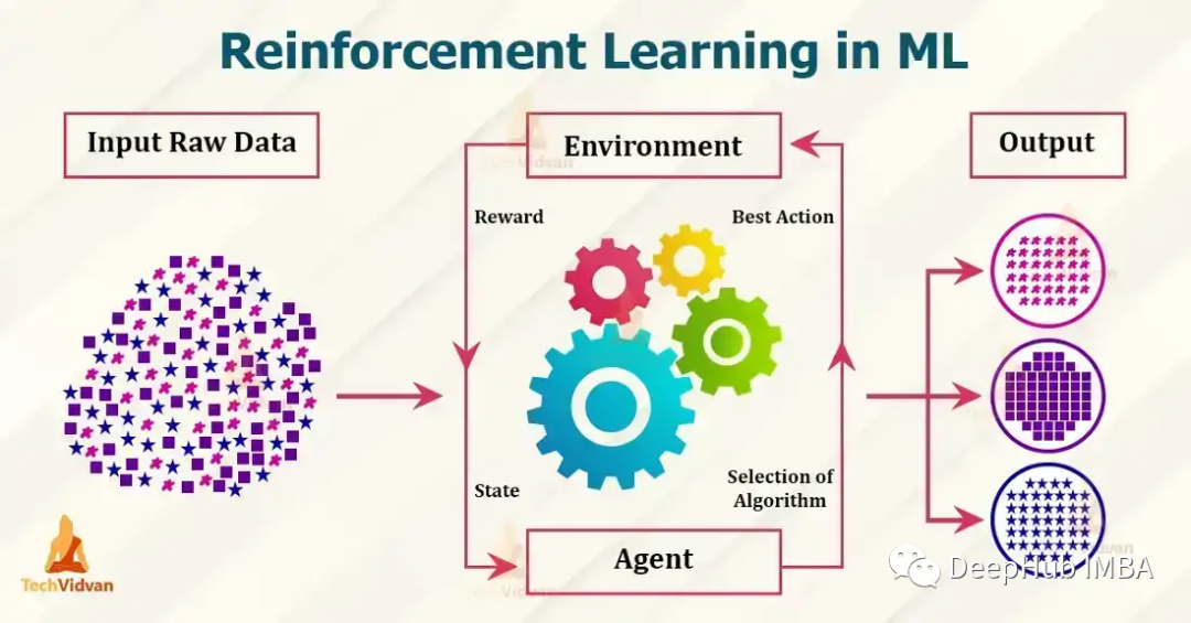
目前流行的强化学习算法包括 Q-learning、SARSA、DDPG、A2C、PPO、DQN 和 TRPO。 这些算法已被用于在游戏、机器人和决策制定等各种应用中,并且这些流行的算法还在不断发展和改进,本文我们将对其做一个简单的介绍。
目前流行的强化学习算法包括 Q-learning、SARSA、DDPG、A2C、PPO、DQN 和 TRPO。 这些算法已被用于在游戏、机器人和决策制定等各种应用中,并且这些流行的算法还在不断发展和改进,本文我们将对其做一个简单的介绍。
1、Q-learning
Q-learning:Q-learning 是一种无模型、非策略的强化学习算法。 它使用 Bellman 方程估计最佳动作值函数,该方程迭代地更新给定状态动作对的估计值。 Q-learning 以其简单性和处理大型连续状态空间的能力而闻名。
下面是一个使用 Python 实现 Q-learning 的简单示例:
import numpy as np

 # Define the Q-table and the learning rate
 Q = np.zeros((state_space_size, action_space_size))
 alpha = 0.1

 # Define the exploration rate and discount factor
 epsilon = 0.1
 gamma = 0.99

 for episode in range(num_episodes):
     current_state = initial_state
     while not done:
         # Choose an action using an epsilon-greedy policy
         if np.random.uniform(0, 1) < epsilon:
             action = np.random.randint(0, action_space_size)
         else:
             action = np.argmax(Q[current_state])

         # Take the action and observe the next state and reward
         next_state, reward, done = take_action(current_state, action)

         # Update the Q-table using the Bellman equation
         Q[current_state, action] = Q[current_state, action] + alpha * (reward + gamma * np.max(Q[next_state]) - Q[current_state, action])

         current_state = next_state
上面的示例中,state_space_size 和 action_space_size 分别是环境中的状态数和动作数。 num_episodes 是要为运行算法的轮次数。 initial_state 是环境的起始状态。 take_action(current_state, action) 是一个函数,它将当前状态和一个动作作为输入,并返回下一个状态、奖励和一个指示轮次是否完成的布尔值。
在 while 循环中,使用 epsilon-greedy 策略根据当前状态选择一个动作。 使用概率 epsilon选择一个随机动作,使用概率 1-epsilon选择对当前状态具有最高 Q 值的动作。
采取行动后,观察下一个状态和奖励,使用Bellman方程更新q。 并将当前状态更新为下一个状态。这只是 Q-learning 的一个简单示例,并未考虑 Q-table 的初始化和要解决的问题的具体细节。
2、SARSA
SARSA:SARSA 是一种无模型、基于策略的强化学习算法。 它也使用Bellman方程来估计动作价值函数,但它是基于下一个动作的期望值,而不是像 Q-learning 中的最优动作。 SARSA 以其处理随机动力学问题的能力而闻名。
import numpy as np

 # Define the Q-table and the learning rate
 Q = np.zeros((state_space_size, action_space_size))
 alpha = 0.1

 # Define the exploration rate and discount factor
 epsilon = 0.1
 gamma = 0.99

 for episode in range(num_episodes):
     current_state = initial_state
     action = epsilon_greedy_policy(epsilon, Q, current_state)
     while not done:
         # Take the action and observe the next state and reward
         next_state, reward, done = take_action(current_state, action)
         # Choose next action using epsilon-greedy policy
         next_action = epsilon_greedy_policy(epsilon, Q, next_state)
         # Update the Q-table using the Bellman equation
         Q[current_state, action] = Q[current_state, action] + alpha * (reward + gamma * Q[next_state, next_action] - Q[current_state, action])
         current_state = next_state
         action = next_action
state_space_size和action_space_size分别是环境中的状态和操作的数量。num_episodes是您想要运行SARSA算法的轮次数。Initial_state是环境的初始状态。take_action(current_state, action)是一个将当前状态和作为操作输入的函数,并返回下一个状态、奖励和一个指示情节是否完成的布尔值。
在while循环中,使用在单独的函数epsilon_greedy_policy(epsilon, Q, current_state)中定义的epsilon-greedy策略来根据当前状态选择操作。使用概率 epsilon选择一个随机动作,使用概率 1-epsilon对当前状态具有最高 Q 值的动作。
上面与Q-learning相同,但是采取了一个行动后,在观察下一个状态和奖励时它然后使用贪心策略选择下一个行动。并使用Bellman方程更新q表。
3、DDPG
DDPG 是一种用于连续动作空间的无模型、非策略算法。 它是一种actor-critic算法,其中actor网络用于选择动作,而critic网络用于评估动作。 DDPG 对于机器人控制和其他连续控制任务特别有用。
import numpy as np
 from keras.models import Model, Sequential
 from keras.layers import Dense, Input
 from keras.optimizers import Adam

 # Define the actor and critic models
 actor = Sequential()
 actor.add(Dense(32, input_dim=state_space_size, activation='relu'))
 actor.add(Dense(32, activation='relu'))
 actor.add(Dense(action_space_size, activation='tanh'))
 actor.compile(loss='mse', optimizer=Adam(lr=0.001))

 critic = Sequential()
 critic.add(Dense(32, input_dim=state_space_size, activation='relu'))
 critic.add(Dense(32, activation='relu'))
 critic.add(Dense(1, activation='linear'))
 critic.compile(loss='mse', optimizer=Adam(lr=0.001))

 # Define the replay buffer
 replay_buffer = []

 # Define the exploration noise
 exploration_noise = OrnsteinUhlenbeckProcess(size=action_space_size, theta=0.15, mu=0, sigma=0.2)

 for episode in range(num_episodes):
     current_state = initial_state
     while not done:
         # Select an action using the actor model and add exploration noise
         action = actor.predict(current_state)[0] + exploration_noise.sample()
         action = np.clip(action, -1, 1)

         # Take the action and observe the next state and reward
         next_state, reward, done = take_action(current_state, action)

         # Add the experience to the replay buffer
         replay_buffer.append((current_state, action, reward, next_state, done))

         # Sample a batch of experiences from the replay buffer
         batch = sample(replay_buffer, batch_size)

         # Update the critic model
         states = np.array([x[0] for x in batch])
         actions = np.array([x[1] for x in batch])
         rewards = np.array([x[2] for x in batch])
         next_states = np.array([x[3] for x in batch])

         target_q_values = rewards + gamma * critic.predict(next_states)
         critic.train_on_batch(states, target_q_values)

         # Update the actor model
         action_gradients = np.array(critic.get_gradients(states, actions))
         actor.train_on_batch(states, action_gradients)

         current_state = next_state
在本例中,state_space_size和action_space_size分别是环境中的状态和操作的数量。num_episodes是轮次数。Initial_state是环境的初始状态。Take_action (current_state, action)是一个函数,它接受当前状态和操作作为输入,并返回下一个操作。
4、A2C
A2C(Advantage Actor-Critic)是一种有策略的actor-critic算法,它使用Advantage函数来更新策略。 该算法实现简单,可以处理离散和连续的动作空间。
import numpy as np
 from keras.models import Model, Sequential
 from keras.layers import Dense, Input
 from keras.optimizers import Adam
 from keras.utils import to_categorical

 # Define the actor and critic models
 state_input = Input(shape=(state_space_size,))
 actor = Dense(32, activation='relu')(state_input)
 actor = Dense(32, activation='relu')(actor)
 actor = Dense(action_space_size, activation='softmax')(actor)
 actor_model = Model(inputs=state_input, outputs=actor)
 actor_model.compile(loss='categorical_crossentropy', optimizer=Adam(lr=0.001))

 state_input = Input(shape=(state_space_size,))
 critic = Dense(32, activation='relu')(state_input)
 critic = Dense(32, activation='relu')(critic)
 critic = Dense(1, activation='linear')(critic)
 critic_model = Model(inputs=state_input, outputs=critic)
 critic_model.compile(loss='mse', optimizer=Adam(lr=0.001))

 for episode in range(num_episodes):
     current_state = initial_state
     done = False
     while not done:
         # Select an action using the actor model and add exploration noise
         action_probs = actor_model.predict(np.array([current_state]))[0]
         action = np.random.choice(range(action_space_size), p=action_probs)

         # Take the action and observe the next state and reward
         next_state, reward, done = take_action(current_state, action)

         # Calculate the advantage
         target_value = critic_model.predict(np.array([next_state]))[0][0]
         advantage = reward + gamma * target_value - critic_model.predict(np.array([current_state]))[0][0]

         # Update the actor model
         action_one_hot = to_categorical(action, action_space_size)
         actor_model.train_on_batch(np.array([current_state]), advantage * action_one_hot)

         # Update the critic model
         critic_model.train_on_batch(np.array([current_state]), reward + gamma * target_value)

         current_state = next_state
在这个例子中,actor模型是一个神经网络,它有2个隐藏层,每个隐藏层有32个神经元,具有relu激活函数,输出层具有softmax激活函数。critic模型也是一个神经网络,它有2个隐含层,每层32个神经元,具有relu激活函数,输出层具有线性激活函数。
使用分类交叉熵损失函数训练actor模型,使用均方误差损失函数训练critic模型。动作是根据actor模型预测选择的,并添加了用于探索的噪声。
5、PPO
PPO(Proximal Policy Optimization)是一种策略算法,它使用信任域优化的方法来更新策略。 它在具有高维观察和连续动作空间的环境中特别有用。 PPO 以其稳定性和高样品效率而著称。
import numpy as np
 from keras.models import Model, Sequential
 from keras.layers import Dense, Input
 from keras.optimizers import Adam

 # Define the policy model
 state_input = Input(shape=(state_space_size,))
 policy = Dense(32, activation='relu')(state_input)
 policy = Dense(32, activation='relu')(policy)
 policy = Dense(action_space_size, activation='softmax')(policy)
 policy_model = Model(inputs=state_input, outputs=policy)

 # Define the value model
 value_model = Model(inputs=state_input, outputs=Dense(1, activation='linear')(policy))

 # Define the optimizer
 optimizer = Adam(lr=0.001)

 for episode in range(num_episodes):
     current_state = initial_state
     while not done:
         # Select an action using the policy model
         action_probs = policy_model.predict(np.array([current_state]))[0]
         action = np.random.choice(range(action_space_size), p=action_probs)

         # Take the action and observe the next state and reward
         next_state, reward, done = take_action(current_state, action)

         # Calculate the advantage
         target_value = value_model.predict(np.array([next_state]))[0][0]
         advantage = reward + gamma * target_value - value_model.predict(np.array([current_state]))[0][0]

         # Calculate the old and new policy probabilities
         old_policy_prob = action_probs[action]
         new_policy_prob = policy_model.predict(np.array([next_state]))[0][action]

         # Calculate the ratio and the surrogate loss
         ratio = new_policy_prob / old_policy_prob
         surrogate_loss = np.minimum(ratio * advantage, np.clip(ratio, 1 - epsilon, 1 + epsilon) * advantage)

         # Update the policy and value models
         policy_model.trainable_weights = value_model.trainable_weights
         policy_model.compile(optimizer=optimizer, loss=-surrogate_loss)
         policy_model.train_on_batch(np.array([current_state]), np.array([action_one_hot]))
         value_model.train_on_batch(np.array([current_state]), reward + gamma * target_value)

         current_state = next_state
6、DQN
DQN(深度 Q 网络)是一种无模型、非策略算法,它使用神经网络来逼近 Q 函数。 DQN 特别适用于 Atari 游戏和其他类似问题,其中状态空间是高维的,并使用神经网络近似 Q 函数。
import numpy as np
 from keras.models import Sequential
 from keras.layers import Dense, Input
 from keras.optimizers import Adam
 from collections import deque

 # Define the Q-network model
 model = Sequential()
 model.add(Dense(32, input_dim=state_space_size, activation='relu'))
 model.add(Dense(32, activation='relu'))
 model.add(Dense(action_space_size, activation='linear'))
 model.compile(loss='mse', optimizer=Adam(lr=0.001))

 # Define the replay buffer
 replay_buffer = deque(maxlen=replay_buffer_size)

 for episode in range(num_episodes):
     current_state = initial_state
     while not done:
         # Select an action using an epsilon-greedy policy
         if np.random.rand() < epsilon:
             action = np.random.randint(0, action_space_size)
         else:
             action = np.argmax(model.predict(np.array([current_state]))[0])

         # Take the action and observe the next state and reward
         next_state, reward, done = take_action(current_state, action)

         # Add the experience to the replay buffer
         replay_buffer.append((current_state, action, reward, next_state, done))

         # Sample a batch of experiences from the replay buffer
         batch = random.sample(replay_buffer, batch_size)

         # Prepare the inputs and targets for the Q-network
         inputs = np.array([x[0] for x in batch])
         targets = model.predict(inputs)
         for i, (state, action, reward, next_state, done) in enumerate(batch):
             if done:
                 targets[i, action] = reward
             else:
                 targets[i, action] = reward + gamma * np.max(model.predict(np.array([next_state]))[0])

         # Update the Q-network
         model.train_on_batch(inputs, targets)

         current_state = next_state
上面的代码,Q-network有2个隐藏层,每个隐藏层有32个神经元,使用relu激活函数。该网络使用均方误差损失函数和Adam优化器进行训练。
7、TRPO
TRPO (Trust Region Policy Optimization)是一种无模型的策略算法,它使用信任域优化方法来更新策略。 它在具有高维观察和连续动作空间的环境中特别有用。
TRPO 是一个复杂的算法,需要多个步骤和组件来实现。TRPO不是用几行代码就能实现的简单算法。
所以我们这里使用实现了TRPO的现有库,例如OpenAI Baselines,它提供了包括TRPO在内的各种预先实现的强化学习算法,。
要在OpenAI Baselines中使用TRPO,我们需要安装:
pip install baselines然后可以使用baselines库中的trpo_mpi模块在你的环境中训练TRPO代理,这里有一个简单的例子:
import gym
 from baselines.common.vec_env.dummy_vec_env import DummyVecEnv
 from baselines.trpo_mpi import trpo_mpi

 #Initialize the environment
 env = gym.make("CartPole-v1")
 env = DummyVecEnv([lambda: env])

 # Define the policy network
 policy_fn = mlp_policy

 #Train the TRPO model
 model = trpo_mpi.learn(env, policy_fn, max_iters=1000)
我们使用Gym库初始化环境。然后定义策略网络,并调用TRPO模块中的learn()函数来训练模型。
还有许多其他库也提供了TRPO的实现,例如TensorFlow、PyTorch和RLLib。下面时一个使用TF 2.0实现的样例
import tensorflow as tf
 import gym

 # Define the policy network
 class PolicyNetwork(tf.keras.Model):
     def __init__(self):
         super(PolicyNetwork, self).__init__()
         self.dense1 = tf.keras.layers.Dense(16, activation='relu')
         self.dense2 = tf.keras.layers.Dense(16, activation='relu')
         self.dense3 = tf.keras.layers.Dense(1, activation='sigmoid')

     def call(self, inputs):
         x = self.dense1(inputs)
         x = self.dense2(x)
         x = self.dense3(x)
         return x

 # Initialize the environment
 env = gym.make("CartPole-v1")

 # Initialize the policy network
 policy_network = PolicyNetwork()

 # Define the optimizer
 optimizer = tf.optimizers.Adam()

 # Define the loss function
 loss_fn = tf.losses.BinaryCrossentropy()

 # Set the maximum number of iterations
 max_iters = 1000

 # Start the training loop
 for i in range(max_iters):
     # Sample an action from the policy network
     action = tf.squeeze(tf.random.categorical(policy_network(observation), 1))

     # Take a step in the environment
     observation, reward, done, _ = env.step(action)

     with tf.GradientTape() as tape:
         # Compute the loss
         loss = loss_fn(reward, policy_network(observation))

     # Compute the gradients
     grads = tape.gradient(loss, policy_network.trainable_variables)

     # Perform the update step
     optimizer.apply_gradients(zip(grads, policy_network.trainable_variables))

     if done:
         # Reset the environment
         observation = env.reset()
在这个例子中,我们首先使用TensorFlow的Keras API定义一个策略网络。然后使用Gym库和策略网络初始化环境。然后定义用于训练策略网络的优化器和损失函数。
在训练循环中,从策略网络中采样一个动作,在环境中前进一步,然后使用TensorFlow的GradientTape计算损失和梯度。然后我们使用优化器执行更新步骤。
这是一个简单的例子,只展示了如何在TensorFlow 2.0中实现TRPO。TRPO是一个非常复杂的算法,这个例子没有涵盖所有的细节,但它是试验TRPO的一个很好的起点。
以上就是我们总结的7个常用的强化学习算法,这些算法并不相互排斥,通常与其他技术(如值函数逼近、基于模型的方法和集成方法)结合使用,可以获得更好的结果。
Recommend
About Joyk
Aggregate valuable and interesting links.
Joyk means Joy of geeK