

对循环神经网络参数的理解|LSTM RNN Input_size Batch Sequence - 孤飞
source link: https://www.cnblogs.com/ranxi169/p/16754873.html
Go to the source link to view the article. You can view the picture content, updated content and better typesetting reading experience. If the link is broken, please click the button below to view the snapshot at that time.
在很多博客和知乎中我看到了许多对于pytorch框架中RNN接口的一些解析,但都较为浅显甚至出现一些不准确的理解,在这里我想阐述下我对于pytorch中RNN接口的参数的理解。
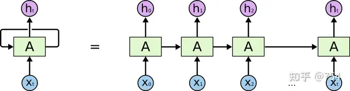
我们经常看到的RNN网络是如图下所示:
RNN的
1. timestep训练过程
这个左边图中间循环的箭头难以理解,所以将其按照时间轴展开成多个单元。
但是!!!!
网络只有一个,网络只有一个,网络只有一个, 并不是想右边那样画的。右边的图只不过是不同时刻的输入。因为每个时刻RNN会产生两个输出,一个output和一个state(state是输入向下一个时序的结果),上一个时刻state和当前作为输入给当前网络,就如右图所示。上图很容易造成了误解。
比如我们需要预测一个sin函数,那么我们会用x的坐标去预测y,batchsize=1(batch_size的问题较为复杂,后续会聊),timestep(sequence的长度)为5,特征为1(只有x坐标),所以整个训练过程是这样的,我们预备出5个坐标,一个一个依次放入到网络中,初始化的h0是0,然后会得到h1,去得到h2,用h2和x3去得到h4,以此类推。。。我们其实只要看上图的左边,不要被右图给搞混,只有一个网络结构而已。只是不停的放入不停的迭代。
2. batch理解
网上对batch的理解鱼龙混杂,什么样的解释都有,这里我要阐述我的观点,用一个博客上的例子,
给定一个长序列,序列中的每一个值,也都由一个很长的向量(或矩阵)表示。把序列从前往后理解为时间维度,那么timestep就是指的这个维度中的值,如果timestep=n,就是用序列内的n个向量(或矩阵)预测一个值,下图的timestep为2。
而对于每一个向量来说,它本身有一个空间维度(如长度),那么Batchsize就是这个空间维度上的概念。
比如一共有5个字母ABCDE,它们分别如此表示:
A:1 1 1 1 1
B:2 2 2 2 2
C:3 3 3 3 3
D:4 4 4 4 4
E:5 5 5 5 5
| X | Y |
|---|---|
| AB | C |
| BC | D |
| CD | E |
下面我们只看第一对数据:AB-C
t=0,A进入训练,生成h(0)
t=1,B进入训练,生成h(1)
如果我们分batch的话,设batch=2,那就AB-C, BC-D一起放入训练,同时平均loss之后经过一次backward更新超参数,由于超参数的方法更新很多,可能是类似于加权的平均。
这样或许很抽象,于是我我以文本数据为例画了一张图

3. hidden_size理解
hidden_size类似于全连接网络的结点个数,hidden_size的维度等于hn的维度,这就是每个时间输出的维度结果。我们的hidden_size是自己定的,根据炼丹得到最佳结果。
为什么我们的input_size可以和hidden_size不同呢,因为超参数已经帮我们完成了升维或降维,如下图(超参数计算流程)。

此时我引用正弦预测例子,后续会展示代码,其中input_size=1,hidden_size=50。
我们可以得到以下结果:

代码附下:
1 2 3 4 5 6 7 8 9 10 11 12 13 14 15 16 17 18 19 20 21 22 23 24 25 26 27 28 29 30 31 32 33 34 35 36 37 38 39 40 41 42 43 44 45 46 47 48 49 50 51 52 53 54 55 56 57 58 59 60 61 62 63 64 65 66 67 68 69 70 71 72 73 74 75 76 77 78 79 80 81 82 83 84 85 86 87 88 89 90 91 92 93 94 95 96 97 98 99 100 101 102 103 104 105 106 107 108 109 110 111 112 113 114 115 116 117 118import numpy as np import pandas as pd import torch import torch.nn as nn import matplotlib.pyplot as plt # %matplotlib inline # 跟matlab差不多 返回一个1维张量,包含在区间start和end上均匀间隔的step个点。 # torch.linspace(start, end, steps, out=None) → Tensor x = torch.linspace(0,799,800) y = torch.sin(x*2*3.1416/40) plt.figure(figsize=(12,4)) plt.xlim(-10,801) plt.grid(True) plt.xlabel("x") plt.ylabel("sin") plt.title("Sin plot") plt.plot(y.numpy(),color='#8000ff') plt.show() test_size = 40 train_set = y[:-test_size]#前760个数 test_set = y[-test_size:]#后40个数 plt.figure(figsize=(12,4)) plt.xlim(-10,801) plt.grid(True) plt.xlabel("x") plt.ylabel("sin") plt.title("Sin plot") plt.plot(train_set.numpy(),color='#8000ff') plt.plot(range(760,800),test_set.numpy(),color="#ff8000") plt.show() # 在使用LSTM模型时,我们将训练序列分为一系列重叠的窗口。用于比较的标签是序列中的下一个值。【滑动窗口】 # 例如,如果我们有一系列12条记录,窗口大小为3,我们将[x1, x2, x3]送入模型,并将预测值与x4比较。 # 然后我们回溯,更新参数,将[x2, x3, x4]输入模型,并将预测结果与x5进行比较。 # 为了简化这个过程,我定义了一个函数input_data(seq,ws),创建了一个(seq,labels)图元的列表。 # 如果ws是窗口大小,那么(seq,labels)图元的总数将是len(series)-ws。 def input_data(seq, ws): out = [] L = len(seq) for i in range(L - ws): window = seq[i:i + ws] label = seq[i + ws:i + ws + 1] out.append((window, label)) return out # The length of x = 800 # The length of train_set = 800 - 40 = 760 # The length of train_data = 760 - 40 - 720 window_size = 40 train_data = input_data(train_set, window_size) len(train_data) train_data[0]#40个滑动窗口,作为一个输入 class LSTM(nn.Module): def __init__(self, input_size=1, hidden_size=50, out_size=1): super().__init__() self.hidden_size = hidden_size self.lstm = nn.LSTM(input_size, hidden_size) self.linear = nn.Linear(hidden_size, out_size) self.hidden = (torch.zeros(1, 1, hidden_size), torch.zeros(1, 1, hidden_size)) def forward(self, seq): lstm_out, self.hidden = self.lstm(seq.view(len(seq), 1, -1), self.hidden) pred = self.linear(lstm_out.view(len(seq), -1)) return pred[-1] torch.manual_seed(42) model = LSTM() criterion = nn.MSELoss() optimizer = torch.optim.SGD(model.parameters(), lr=0.01) epochs = 10 future = 40 for i in range(epochs): for seq, y_train in train_data: optimizer.zero_grad() model.hidden = (torch.zeros(1, 1, model.hidden_size), torch.zeros(1, 1, model.hidden_size)) y_pred = model(seq) loss = criterion(y_pred, y_train) loss.backward() optimizer.step() print(f"Epoch {i} Loss: {loss.item()}") preds = train_set[-window_size:].tolist() for f in range(future): seq = torch.FloatTensor(preds[-window_size:]) with torch.no_grad(): model.hidden = (torch.zeros(1, 1, model.hidden_size), torch.zeros(1, 1, model.hidden_size)) preds.append(model(seq).item()) loss = criterion(torch.tensor(preds[-window_size:]), y[760:]) print(f"Performance on test range: {loss}") plt.figure(figsize=(12, 4)) plt.xlim(700, 801) plt.grid(True) plt.plot(y.numpy(), color='#8000ff') plt.plot(range(760, 800), preds[window_size:], color='#ff8000') plt.show()
参考文章:https://zhuanlan.zhihu.com/p/460282865
原创作者:孤飞-博客园
个人博客:https://blog.onefly.top
Recommend
About Joyk
Aggregate valuable and interesting links.
Joyk means Joy of geeK