Python 系列：测量程序的运行时间

Python 系列：测量程序的运行时间

说到测量程序的运行时间这件事，我最早的做法是在桌上摆个手机，打开秒表应用，右手在命令行里敲回车的同时左手启动秒表，看屏幕上程序跑完后再马上按停秒表，最后在纸上记下时间。后来我在 Linux 上学会了在命令开头添加一个 time，终于摆脱了手动计时的原始操作。这次就想总结一下迄今为止我用过的那些测量时间的工具/代码。

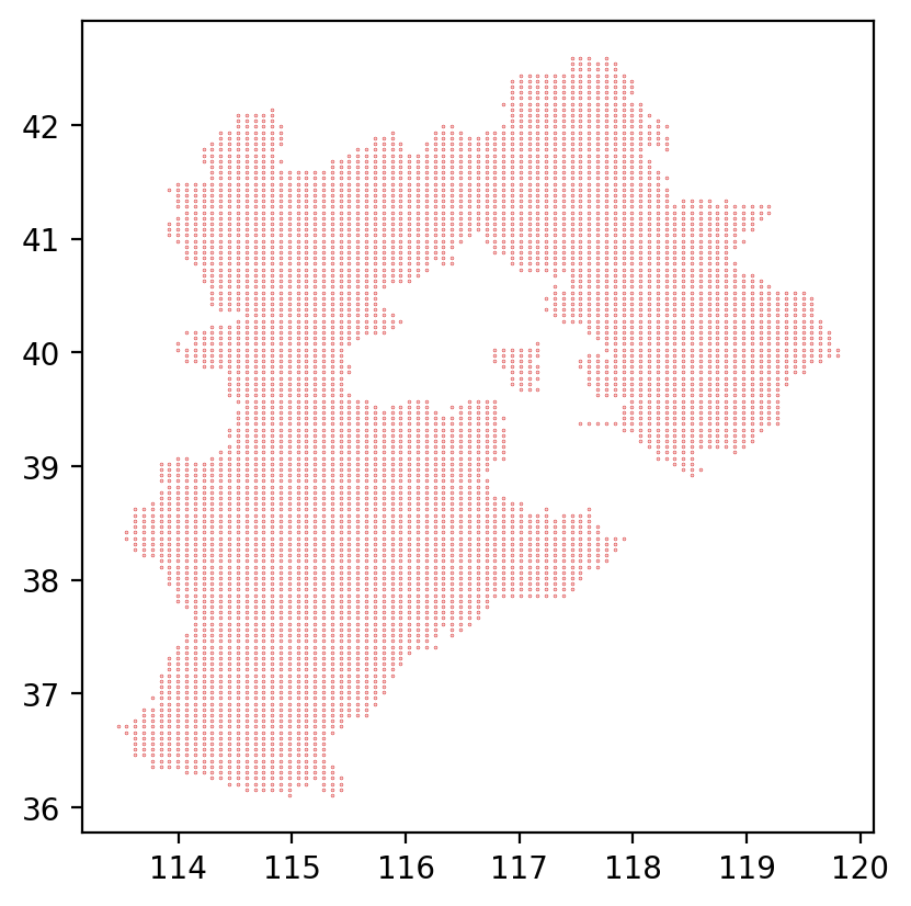
测试代码是读取河北省省界的 GeoJSON 文件，利用射线法判断网格点有没有落入省界内部，最后通过 Matplotlib 画出示意图并保存。GeoJSON 数据来自阿里云的 DataV.GeoAtlas。代码 test.py 的内容如下

import json

import numpy as np
import matplotlib.pyplot as plt

def contain(polygon, x, y):
    '''判断点是否落入多边形中.'''
    if polygon['type'] == 'Polygon':
        coords_polygons = [polygon['coordinates']]
    elif polygon['type'] == 'MultiPolygon':
        coords_polygons = polygon['coordinates']
    else:
        raise ValueError('输入不是多边形')

    # 对每个多边形应用射线法.
    for coords_polygon in coords_polygons:
        flag = False
        for coords_ring in coords_polygon:
            for i in range(len(coords_ring) - 1):
                x0, y0 = coords_ring[i]
                x1, y1 = coords_ring[i + 1]
                if y0 < y <= y1 or y1 < y <= y0:
                    if x < (x1 - x0) / (y1 - y0) * (y - y0) + x0:
                        flag = not flag
        if flag:
            return flag

    return False

def main():
    with open('河北省.json', encoding='utf-8') as f:
        geoj = json.load(f)
        hebei = geoj['features'][0]['geometry']

    xs = []
    ys = []
    for x in np.linspace(110, 125, 200):
        for y in np.linspace(35, 45, 200):
            if contain(hebei, x, y):
                xs.append(x)
                ys.append(y)

    fig, ax = plt.subplots()
    ax.set_aspect('equal')
    ax.plot(xs, ys, 'o', c='C3', ms=0.2)
    fig.savefig('hebei.png', dpi=200, bbox_inches='tight')
    plt.close(fig)

if __name__ == '__main__':
    main()

输出图片为

Linux 的 time

在 Linux 的 Bash 中通过在命令前加上 time，即可在命令执行结束后打印出三种耗时

(base) laptop@zhajiman:/code$ time python test.py

real	0m22.993s
user	0m19.905s
sys		0m0.096s

其中 real 指总耗时（墙上时钟经过的时间，即 wall time），user 指用户态代码耗费的 CPU 时间，sys 指系统态代码耗费的 CPU 时间。一般看 real 的数值即可，关于三种时间的解释可见 linux time命令详解与坑。

Windows 的 Measure-Command

Windows 中类似的命令是 Powershell 的 Measure-Command 命令

(base) PS D:\code> Measure-Command {python test.py}

Days              : 0
Hours             : 0
Minutes           : 0
Seconds           : 16
Milliseconds      : 442
Ticks             : 164424518
TotalDays         : 0.000190306155092593
TotalHours        : 0.00456734772222222
TotalMinutes      : 0.274040863333333
TotalSeconds      : 16.4424518
TotalMilliseconds : 16442.4518

打印出了各种单位的耗时，一般看其中的 TotalSeconds 即可。不过该命令会吞掉 Python 程序本身的打印结果，这时可以通过管道在测量结束后把内容再打印出来

Measure-Command {python test.py | Out-Default}

显然 Linux 的 time 命令用起来要方便的多……

IPython 的魔法命令

IPython 中的 %run 命令可以直接执行脚本文件，加上 -t 参数时会输出耗时

In [1]: %run -t test.py

IPython CPU timings (estimated):
  User   :      16.17 s.
  System :       0.00 s.
Wall time:      16.37 s.

输出结果跟 Linux 的 time 命令很像，不过文档说 Windows 下的 System 时间直接设成了 0。加上 -N <N> 参数可以重复执行 <N> 次，输出里会多出总时间和平均时间之分。

%time

%time 会打印出单条语句或表达式的耗时

In [2]: %time main()
CPU times: total: 16.6 s
Wall time: 16.8 s

结果由 CPU 时间和墙上时间组成。

%timeit

类似 %time，但为了得到精准的测量结果，会自动测量多次，以得到较为准确的平均耗时，还会为打印出来的结果挑选合适的单位（秒、毫秒、微秒等）。例如

In [3]: with open('河北省.json', encoding='utf-8') as f:
   ...:     geoj = json.load(f)
   ...:     hebei = geoj['features'][0]['geometry']
   ...:

In [4]: %timeit contain(hebei, 115, 40)
284 µs ± 4.63 µs per loop (mean ± std. dev. of 7 runs, 1,000 loops each)

%timeit 默认跑 7 组，每组自动设置成了 1000 次循环，最后计算平均耗时和标准差。加上 -n <N> 可以指定循环 <N> 次，-r <R> 可以指定跑 <R> 组。例如测一次 main 函数的耗时

In [5]: %timeit -n 1 -r 1 main()
15.4 s ± 0 ns per loop (mean ± std. dev. of 1 run, 1 loop each)

无论是 %time 还是 %timeit 都有一个缺陷：只能在 IPython 顶层的命名空间中使用。例如我想测试 contain(hebei, x, y) 对于单点的速度，因为变量 hebei 在函数 main 的命名空间里，而外部没有，所以我在使用 %timeit 前又在全局新建了 hebei 变量。我还试过设置断点通过 ipdb 跳到函数内，结果发现此时 %timeit 用不了，不知道读者有没有比较好的解决方法。

标准库的 time 模块

time 和 perf_counter 函数

time 模块的一个主要功能就是获取当前时间，所以只要在想计时的代码块开头获取一次时间，再在结尾获取一次，最后计算二者的差值就能得到代码块的耗时。例如

import time

if __name__ == '__main__':
    t0 = time.time()
    main()
    t1 = time.time()
    dt = t1 - t0
    print(f'{dt:.1f}', 's')

打印结果为 15.4 s。其中 time.time 函数没有参数，在 Windows 和 Linux 平台上调用后返回 Unix 时间戳（自 1970-01-01 00:00:00 UTC 以来的秒数）。这个函数的问题是与系统时间相关联，如果两次调用之间系统时间发生了变动（例如在任务栏里手动修改、联网自动校正等），那么第二次调用的结果也会跟着变化，最后计算出错误的 dt。另外该函数在 Windows 平台的时间分辨率也比较低，会测不准耗时较短的语句。

time.perf_counter 是 Python 3.3 起引入的新函数，名字是 performance counter 之意，即专门用来测量性能（耗时）的计时器。调用后返回的浮点数本身没有明确的意义，只有两次调用时结果的差值有意义，表示过程中经过的秒数。相比 time，perf_counter 的时间分辨率更高，且不受系统时间变动的影响，结果始终保证单调递增。所以在测量程序耗时中更推荐使用 perf_counter。

if __name__ == '__main__':
    t0 = time.perf_counter()
    main()
    t1 = time.perf_counter()
    dt = t1 - t0
    print(f'{dt:.1f}', 's')

另外 time 模块里还有一个 process_time 函数，说是能测量当前进程的用户态和系统态 CPU 时间之和，且不包含睡眠时间（例如调用 time.sleep 函数）。但我测试后发现测出来的时间经常比 perf_counter 的结果要大，实在让人摸不着头脑，所以这里就不多介绍了。

直接在程序中插入 perf_counter 的用法虽然很灵活，但改起来十分麻烦。如果只想测量函数的耗时，使用装饰器语法更方便：无需修改函数体或主程序，只需在定义函数的 def 语句前插入一行，就能为函数增加计时功能。下面编写一个带可选参数的计时装饰器

import time
import functools

def timer(func=None, *, prompt=True, fmt=None, prec=None, out=None):
    '''
    计时用的装饰器.

    Parameters
    ----------
    func : callable
        需要被计时的函数或方法.

    prompt : bool
        是否打印计时结果.

    fmt : str
        打印格式. %n表示函数名, %t表示耗时.

    prec : int
        打印时的小数位数.

    out : list
        收集耗时的列表.
    '''
    if fmt is None:
        fmt = '[%n] %t s'
    if func is None:
        return functools.partial(
            timer, prompt=prompt, fmt=fmt, prec=prec, out=out
        )

    @functools.wraps(func)
    def wrapper(*args, **kwargs):
        t0 = time.perf_counter()
        result = func(*args, **kwargs)
        t1 = time.perf_counter()
        dt = t1 - t0

        # 是否打印结果.
        if prompt:
            st = str(dt) if prec is None else f'{dt:.{prec}f}'
            info = fmt.replace('%n', func.__name__).replace('%t', st)
            print(info)

        # 是否输出到列表中.
        if out is not None:
            out.append(dt)

        return result

    return wrapper

装饰器相关的知识可见 入门Python装饰器。用法是在 main 函数前一行加上 @timer 即可，还可以通过参数控制装饰器的输出

results = []
@timer(fmt='Time spent by %n is %t s', prec=1, out=results)
def main():
    <函数体省略>

Time spent by main is 16.9 s

同时耗时被保存到了全局的 results 列表中。如果想要测量的函数并非定义在当前文件里（例如第三方包里的函数），那么可以通过包装目标函数来实现。例如测量 figsave 方法的用时

timer(prec=1)(fig.savefig)('hebei.png', dpi=200, bbox_inches='tight')

[savefig] 0.148 s

标准库的 cProfile 模块

time 模块适合测量代码块或函数的总耗时，如果想深入了解组成代码的所有函数各占了多长时间，推荐使用标准库的 cProfile 模块。该模块能够对程序进行性能剖析（profile），详尽给出各种函数和方法被调用的次数和耗时。但也因为监控的层级过于深入，会在一定程度上拖慢原程序的运行速度。所以该模块适合分析程序内各部分的相对用时，而不适合做精确的性能比较（benchmark）。

命令行调用

直接在命令行调用会对整个脚本进行测量，无需对代码进行任何修改

python -m cProfile [-o output_file] [-s sort_order] myscript.py

-o 表示将剖析结果输出为二进制文件，如果不给出就将结果以表格的形式打印在屏幕上。-s 表示如果不输出文件，那么可以按 pstats 模块 Stats.sort_stats 方法的规则对打印的表格记录进行排序。由于表格一般巨长无比，所以打印到屏幕上意义不大，我会用管道输出到文本文件后再用编辑器来看。例如在 PowerShell 中可以

python -m cProfile -s cumtime test.py | Out-File -FilePath test.txt 

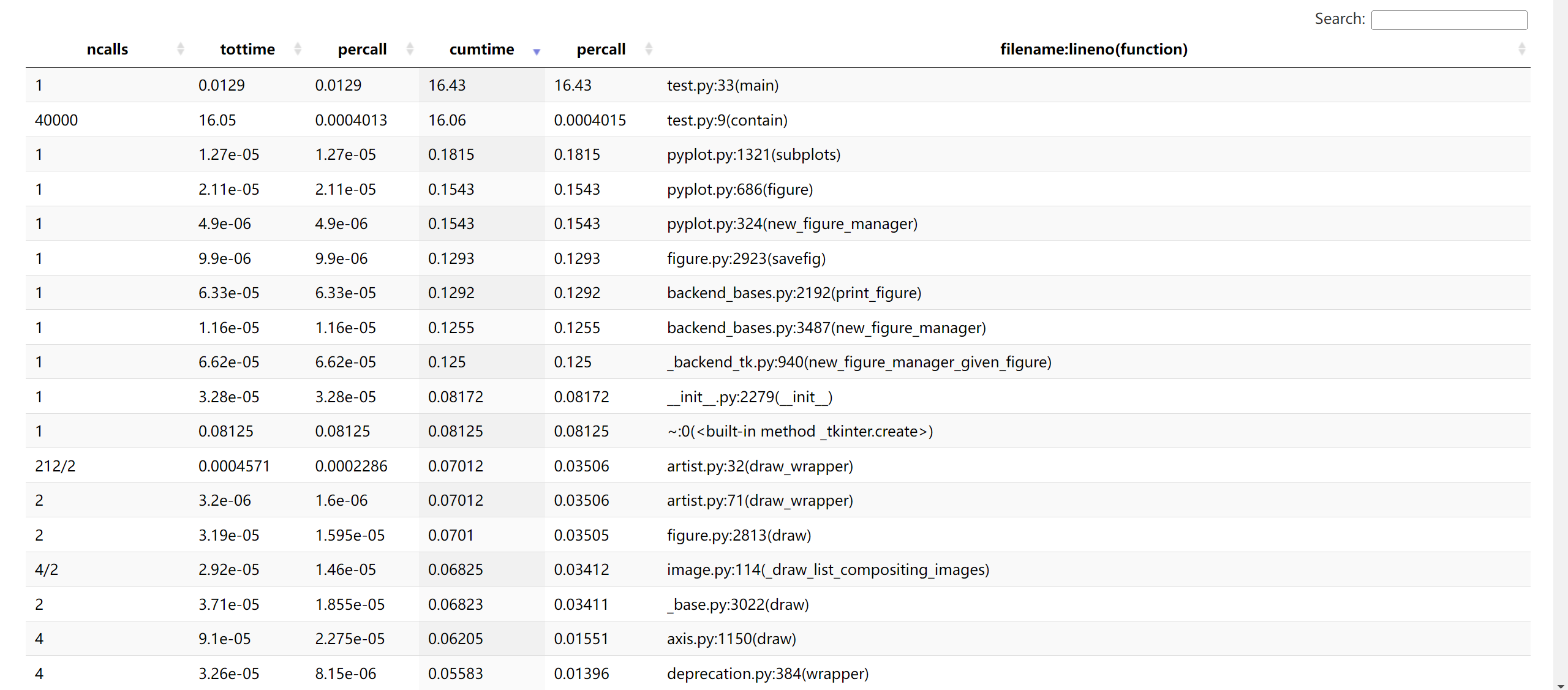
表格前 20 行长这个样子

         3372760 function calls (3338684 primitive calls) in 19.628 seconds

   Ordered by: cumulative time

   ncalls  tottime  percall  cumtime  percall filename:lineno(function)
    782/1    0.003    0.000   19.629   19.629 {built-in method builtins.exec}
        1    0.000    0.000   19.629   19.629 test.py:1(<module>)
        1    0.028    0.028   17.907   17.907 test.py:33(main)
    40000   17.519    0.000   17.532    0.000 test.py:9(contain)
       96    0.003    0.000    3.383    0.035 __init__.py:1(<module>)
   871/15    0.006    0.000    1.760    0.117 <frozen importlib._bootstrap>:1022(_find_and_load)
   868/15    0.004    0.000    1.760    0.117 <frozen importlib._bootstrap>:987(_find_and_load_unlocked)
   833/16    0.004    0.000    1.755    0.110 <frozen importlib._bootstrap>:664(_load_unlocked)
   773/15    0.002    0.000    1.754    0.117 <frozen importlib._bootstrap_external>:877(exec_module)
  1106/16    0.001    0.000    1.754    0.110 <frozen importlib._bootstrap>:233(_call_with_frames_removed)
   535/25    0.001    0.000    1.659    0.066 {built-in method builtins.__import__}
 1086/417    0.002    0.000    1.264    0.003 <frozen importlib._bootstrap>:1053(_handle_fromlist)
2652/2432    0.038    0.000    0.926    0.000 {built-in method builtins.__build_class__}
        1    0.000    0.000    0.883    0.883 pyplot.py:1(<module>)
      101    0.001    0.000    0.690    0.007 artist.py:128(_update_set_signature_and_docstring)

可以看到加了 cProfile 后程序耗时从 16 秒上升至 19 秒，期间共发生 3372760 次函数调用（不算递归的原始调用是 3338684 次）。表格各列的意义如下：

• ncalls：函数调用的次数。正斜杠区分总次数和原始调用。
• tottime：每次调用的耗时之和，但如果函数内调用了其它函数，刨除掉在子函数中经过的时间。
• percall：tottime 除以 ncalls 的值。
• cumtime：每次调用的耗时之和，包含花费在子函数上的时间。
• percall：cumtime 除以原始调用次数的值。
• filename:lineno(function)：函数所在的文件名、定义所在的行号，和函数名。

-s 选项可以按这些列名进行排序，文件名和行号的话用 filename 和 line。表格中总耗时排第一的是内置方法 exec，可能是 cProfile 需要用 exec 执行 test.py 中的语句；第二是作为整个模块的 test.py，再是 main 函数；第四的 contain 函数调用 200 * 200 = 40000 次，耗时 17 秒，说明整个程序中最耗时的操作就是判断点是否落入多边形。而画图相关的函数在表格中的排位并不算高。

程序内调用

如果想要指定测量范围，就需要在程序中显式调用 cProfile 模块。测量单条语句的耗时可以用：

• cProfile.run(command, filename=None, sort=-1)：command 是用字符串表示的 Python 语句，该方法会用 exec 函数执行该语句并测量其耗时。filename 参数用于将结果输出为文件，缺省时会打印出结果表格。sort 参数类似上一节，对打印结果进行排序。
• cProfile.runctx(command, globals, locals, filename=None, sort=-1)：传入 run 的语句仅能引用全局作用域中的对象，而 runctx 可以指定全局作用域和局部作用域的字典。

例如测量 main() 这一句的耗时，输出与上一节类似

import cProfile

if __name__ == '__main__':
    cProfile.run('main()', sort='cumtime')

测量代码块的耗时需要构造 cProfile.Profile 对象，它相当于一个计时器，通过调用方法来开关，会把计时结果保存下来，之后可以选择打印或输出文件。具体方法为：

• enable()：开始测量。
• disable()：结束测量。
• print_stats(sort=-1)：在内部创建一个 Stats 对象并用它打印表格，用 sort 参数进行排序。
• dump_stats(filename)：将测量结果输出到文件。
• run(cmd)：类似 cProfile.run，但没了打印和输出文件功能。
• runctx(cmd, globals, locals)：类似 cProfile.runctx。
• runcall(func, /, *args, **kwargs)：相当于先 enable()，再跑 func(*args, **kwargs)，然后 disable()。

以画图部分的代码块为例，先在开头开启计时器，再在结尾停止计时

profile = cProfile.Profile()
profile.enable()
fig, ax = plt.subplots()
ax.set_aspect('equal')
ax.plot(xs, ys, 'o', c='C3', ms=0.2)
fig.savefig('hebei.png', dpi=200, bbox_inches='tight')
plt.close(fig)
profile.disable()
profile.print_stats('cumtime')

另外 Profile 类支持上下文管理器，允许用 with 语句控制计时器的开关。所以上例可以改写为

with cProfile.Profile() as profile:
    fig, ax = plt.subplots()
    ax.set_aspect('equal')
    ax.plot(xs, ys, 'o', c='C3', ms=0.2)
    fig.savefig('hebei.png', dpi=200, bbox_inches='tight')
    plt.close(fig)
profile.print_stats('cumtime')

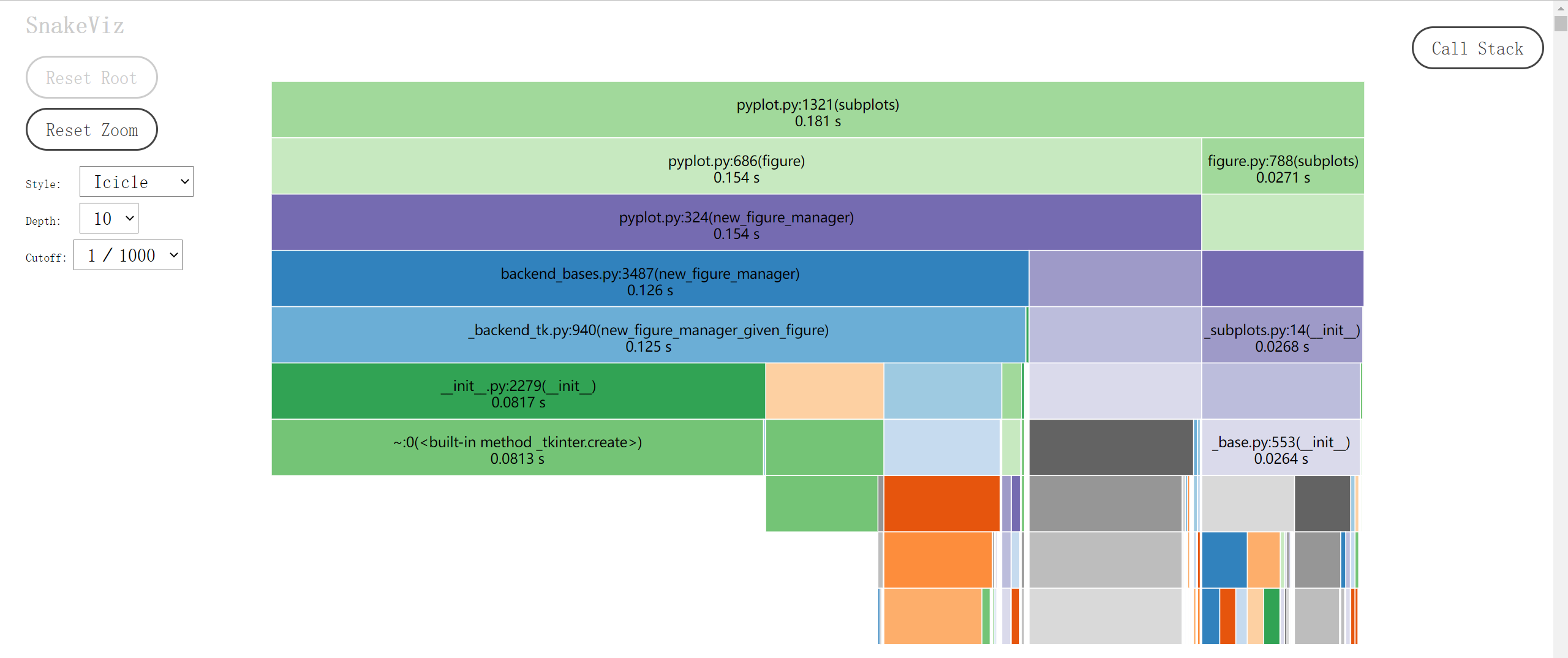
前 20 行结果为，可以看到保存图片的语句耗时最长

         199075 function calls (195323 primitive calls) in 0.454 seconds

   Ordered by: cumulative time

   ncalls  tottime  percall  cumtime  percall filename:lineno(function)
        1    0.000    0.000    0.251    0.251 figure.py:2923(savefig)
        1    0.000    0.000    0.251    0.251 backend_bases.py:2192(print_figure)
        1    0.000    0.000    0.192    0.192 pyplot.py:1321(subplots)
        1    0.000    0.000    0.165    0.165 pyplot.py:686(figure)
        1    0.000    0.000    0.165    0.165 pyplot.py:324(new_figure_manager)
        1    0.000    0.000    0.130    0.130 backend_bases.py:3487(new_figure_manager)
        1    0.000    0.000    0.129    0.129 _backend_tk.py:940(new_figure_manager_given_figure)
        2    0.000    0.000    0.125    0.063 artist.py:71(draw_wrapper)
    212/2    0.001    0.000    0.125    0.063 artist.py:32(draw_wrapper)
        2    0.000    0.000    0.125    0.063 figure.py:2813(draw)
      4/2    0.000    0.000    0.122    0.061 image.py:114(_draw_list_compositing_images)
        2    0.000    0.000    0.122    0.061 _base.py:3022(draw)
        4    0.000    0.000    0.113    0.028 axis.py:1150(draw)
        4    0.000    0.000    0.111    0.028 deprecation.py:384(wrapper)
        2    0.000    0.000    0.109    0.054 backend_bases.py:1595(wrapper)

编写一个测量函数用时并保存结果的装饰器

import cProfile
import functools

def cprofiler(filename):
    '''cProfile的装饰器. 保存结果到指定路径.'''
    def decorator(func):
        @functools.wraps(func)
        def wrapper(*args, **kwargs):
            with cProfile.Profile() as profile:
                result = func(*args, **kwargs)
            profile.dump_stats(filename)
            return result
        return wrapper
    return decorator

使用方法为

@cprofiler('main.prof')
def main():
    <函数体省略>

可视化结果

cProfile 模块输出的二进制文件可以用 pstats 模块的 Stats 类进行读取，它相当于一个表格对象，能对记录进行复杂的排序、只打印前 n 条记录等。还可以直接用记录了测量结果的 Profile 对象构造 Stats 对象。Profile.print_stats 方法其实就是借助 Stats.print_stats 实现的。不过个人觉得这个模块挺鸡肋，不如直接 Profile.print_stats('cumtime') 结合管道导出文本文件，然后再在文本编辑器中查看。

除此之外，另一个直观查看结果的方式就是用第三方包做可视化。这里介绍 snakeviz 包，通过 pip 或 conda 即可安装，使用方法非常简单，在命令行执行

snakeviz main.prof

就能解析 main.prof 文件，在弹出的网页里展示可视化结果。下图是各函数耗时的冰柱图（icicle）：最顶层的长条矩形是被 cProfile.Profile 包裹的 main 函数，下一层则将上一层的矩形细分为不同颜色的子矩形，对应于 main 的函数体中被调用的各种函数，矩形长度正比于耗时。再下一层又会细分上一层的函数调用，如此不断深入，直至某个函数仅由内置语句和函数组成，或调用了其它语言的库文件。最后图片会自上而下形成一个个小山丘，又似冬天屋檐上结成的冰柱，各函数的耗时情况一目了然。Snakeviz 的网页里可以用鼠标点击感兴趣的矩形，会以这个函数为顶层放大冰柱图的细节，之后可以点击左边的 Reset Zoom 按钮返回初始状态。

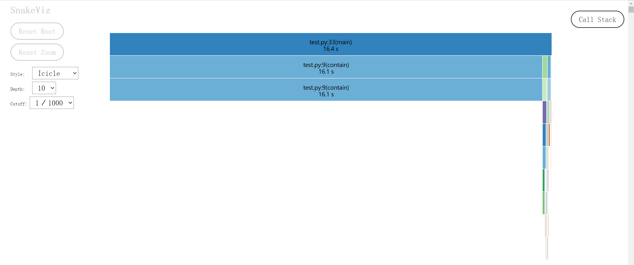
网页下半部分还有表格结果，点击列名以排序，点击行以做出该函数为顶层的冰柱图。这样一来连打印表格的 Profile.print_stats 都可以省去了。

除 snakeviz 外，还有 gprof2dot、flameprof 等工具可选。

line_profiler 模块

cProfile 只能监测函数和方法的耗时，并且会深入到最底层的调用，有时我们并不需要如此详细的信息，只是想了解每一行的耗时。这种情况下第三方模块 line_profiler 可能会更合适，正如它的名字所示，测量的是函数体每一行语句的耗时。同样是 pip 或 conda 安装。

程序内调用

line_profiler.LineProfiler 只提供对函数的测量功能，在构造时需要传入目标函数，也可以后面再添加

from line_profiler import LineProfiler

profile = LineProfiler(f, g)
profile.add_function(h)

常用的方法有：

• run(cmd)：测量一条语句的耗时。但如果语句中不含对目标函数的调用，那就啥也测不到。
• runctx(cmd, globals, locals)：可以传入环境的 run。
• runcall(func, *args, **kw)： 测量 func(*args, **kw) 耗时。当然前提是之前添加过 func 函数。
• enable_by_count()：据文档说是解决了嵌套安全性的 enable。
• disable_by_count()：同上。
• print_stats(self, stream=None, output_unit=None, stripzeros=False)：打印结果，stream 指定输出流（默认屏幕），output_unit 指定结果中的时间单位（后面再解释），stripzeros 指定是否隐藏未被调用的函数。
• dump_stats(self, filename)：以二进制格式导出文件。

以 main 函数为例

if __name__ == '__main__':
    profile = LineProfiler(main)
    profile.enable_by_count()
    main()
    profile.disable_by_count()
    profile.dump_stats('main.lprof')

生成的二进制文件通过下面的命令打印

python -m line_profiler main.lprof

Timer unit: 1e-06 s

Total time: 60.5731 s
File: D:\code\python\profiler\test.py
Function: main at line 34

Line #      Hits         Time  Per Hit   % Time  Line Contents
==============================================================
    34                                           def main():
    35         2         87.8     43.9      0.0      with open('河北省.json', encoding='utf-8') as f:
    36         1        895.7    895.7      0.0          geoj = json.load(f)
    37         1          1.4      1.4      0.0          hebei = geoj['features'][0]['geometry']
    38
    39         1          0.7      0.7      0.0      xs = []
    40         1          0.5      0.5      0.0      ys = []
    41       201        295.5      1.5      0.0      for x in np.linspace(110, 125, 200):
    42     40200      59299.5      1.5      0.1          for y in np.linspace(35, 45, 200):
    43     40000   60157225.0   1503.9     99.3              if contain(hebei, x, y):
    44      5226       9045.1      1.7      0.0                  xs.append(x)
    45      5226       3818.1      0.7      0.0                  ys.append(y)
    46
    47         1     188088.4 188088.4      0.3      fig, ax = plt.subplots()
    48         1         34.6     34.6      0.0      ax.set_aspect('equal')
    49         1       1567.8   1567.8      0.0      ax.plot(xs, ys, 'o', c='C3', ms=0.2)
    50         1     145367.5 145367.5      0.2      fig.savefig('hebei.png', dpi=200, bbox_inches='tight')
    51         1       7339.0   7339.0      0.0      plt.close(fig)

• Line：行号。
• Hits：这一行被“命中”（执行）了几次。
• Time：这一行的总耗时。乘上开头的时间单位 Timer unit 后才是真实数值。
• Per Hit：Time / Hits 的值，表示每次执行的平均耗时。
• % Time：百分数形式的 Time。
• Line Contents：这一行语句的内容。

因为表格内容非常清晰易懂，所以不需要做什么可视化，并且也不会像 cProfile 那样出现一堆见都没见过的函数。令人大跌眼镜的是，被测量的 main 函数耗时从 16 秒暴增至 60 秒。暗示循环语句太多时测量会严重拖慢程序，幸好我们更关心的是 % Time 列的内容，即哪一行占的时间最多。显然 contain 占据了 99.3 %，这提示我们 contain 函数应该是优化的首要对象。

上面的用法还可以改写为

if __name__ == '__main__':
    profile = LineProfiler(main)
    profile.runcall(main)
    profile.print_stats()

然后用管道输出文本结果，这样就可以省去中间的 test.lprof 文件和 python -m 命令。

LineProfiler 类的实例可以直接用作装饰器，会自动通过 add_function 方法添加目标函数。例如

profile = LineProfiler()
@profile
def contain(polygon, x, y):
    <函数体省略>

if __name__ == '__main__':
    main()
    profile.print_stats()

另外也可以自己实现一个保存结果的装饰器

def lprofiler(filename):
    '''line_profiler的装饰器. 保存结果到指定路径.'''
    def decorator(func):
        @functools.wraps(func)
        def wrapper(*args, **kwargs):
            profile = LineProfiler(func)
            result = profile.runcall(func, *args, **kwargs)
            profile.dump_stats(filename)
            return result
        return wrapper
    return decorator

不过自己写的版本有个毛病，反复调用被装饰的函数会重写结果文件，导致无法测量累积用时。

kernprof

kernprof 是 line_profiler 附带的一个脚本，作用是简化调用 LineProfiler 的流程，自动输出结果文件。在命令行里用它代替 Python 命令执行脚本时，会先构造一个名为 profile 的 LineProfiler 对象，并将其注入脚本的命名空间。这样一来脚本开头无需添加 import 语句就能直接引用 profile 变量，接着用它装饰目标函数即可。这也是 line_profiler 文档的推荐用法。例如在脚本中加上一行

@profile
def main():
    <函数体省略>

也不需要写什么 profile.dump_stats(filename)，直接在命令行执行

kernprof -l test.py

就会在当前目录自动生成 test.py.lprof 文件。kernprof 的详细用法可以用 -h 选项查看，下面列举几条常用的：

• -l, --line-by-line：给出时使用 line_profiler，否则使用 cProfile。
• -b, --builtin：是否把 profile 注入脚本。-l 时默认开启。
• -o OUTFILE, --outfile OUTFILE：将结果输出至 OUTFILE 文件。不给出时默认以 脚本名.prof 或 脚本名.lprof 为名保存到当前目录。
• -v, --view：是否顺便打印出结果。

其中 -l 选项提到了可以使用 cProfile，kernprof 对 cProfile.Profile 进行了包装，为其增加了装饰器功能，用法跟前面一样。以测量代码块为例

with profile:
    <代码块省略>

不加 -l，记得加 -b

kernprof -b test.py

会在当前目录自动生成 test.py.prof 文件，接着可以交给 snakeviz 去可视化。

由简到繁总结一下上述工具的使用场景：

• 测量脚本用时：系统命令或 IPython 的 %run。
• 测量函数用时：IPython 的 %time、%timeit。
• 测量代码块用时：time 模块。
• 测量函数每一行的用时：line_profiler 模块。
• 测量函数或代码块所有调用的用时：cProfile 模块。

因笔者对 Jupyter Notebook 不熟，所以没能介绍 %time 和 %timeit 的 cell 版本。另外也没能测试多进程下各工具的表现，专门提到这个是因为笔者在实际操作中经历过 line_profiler 和 kernprof 在多进程脚本中失效的现象。以后有机会再总结一下这些内容。

Point-In-Polygon Algorithm — Determining Whether A Point Is Inside A Complex Polygon

Windows equivalent to UNIX “time” command

IPython: Built-in magic commands

Python Docs: time

Understanding time.perf_counter() and time.process_time()

关于python中time.perf_counter() 与 time.process_time()分析与疑问

Python Cookbook: 9.6 带可选参数的装饰器

Python Docs: The Python Profilers

SNAKEVIZ

pyutils/line_profiler

Python优化第一步: 性能分析实践

好用的 Python Profile（性能/耗时分析）工具