rgee example #1: Creating static and interactive maps

What is rgee?

rgee is a bindings package for Google Earth Engine (GEE). As you probably know, GEE is a cloud-based platform that allows users to have an easy access to a petabyte-scale archive of remote sensing data and run geospatial analysis on Google’s infrastructure. While the use of GEE has spread around different earth sciences communities. It has been relegated from R spatial users due that Google only offers native support for Python and JavaScript programming languages.

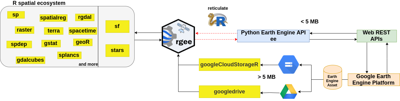
To offer support for R, rgee wraps the Earth Engine Python API using reticulate. In contrast with native client libraries, rgee adds several new features such as (i) new I/O design, (ii) interactive map display, (iii) easy extraction of time series, (iv) asset management interface, and (v) metadata display. The image bellow show you how rgee currently works.

Install the rgee package from GitHub is quite simple, you just have to run in your R console as follows:

remotes::install_github("r-spatial/rgee")

Prior to using rgee you will need to install a Python version higher than 3.5 in your system. rgee counts with an installation function (ee_install) which helps to setup rgee correctly:

library(rgee)
ee_install()

For further information of rgee. Visit the website: https://r-spatial.github.io/rgee/

Tutorial #1: Global Land Surface Temperature map

Load the necessary libraries

library(mapedit) # (OPTIONAL) Interactive editing of vector data
library(raster)  # Manipulate raster data
library(scales)  # Scale functions for visualization
library(cptcity)  # cptcity color gradients!
library(tmap)    # Thematic Map Visualization <3
library(rgee)    # Bindings for Earth Engine

Initialize your Earth Engine session

ee_Initialize()

Search into the Earth Engine’s public data archive. We will use the MOD11A1 V6 product, it provides daily land surface temperature (LST) and emissivity values in a 1200 x 1200 kilometer grid.

ee_search_dataset() %>%
  ee_search_tags("mod11a1") %>%
  ee_search_display()

Load the MOD11A1 ImageCollection. Filter it, for instance, for a specific month, and create a mean composite.

dataset <- ee$ImageCollection("MODIS/006/MOD11A1")$
  filter(ee$Filter$date('2020-01-01', '2020-01-31'))$
  mean()

The ‘LST_Day_1km’ is the band that contains daytime land surface temperature values. We select it and transform the values from kelvin to celsius degrees.

landSurfaceTemperature <- dataset$
  select("LST_Day_1km")$
  multiply(0.02)$
  subtract(273.15)

If you feel weird using the dollar sign operator (‘$’) in this way. Try using pipes (%>%) instead.

landSurfaceTemperature <- dataset %>%
  ee$Image$select("LST_Day_1km") %>%
  ee$Image$multiply(0.02) %>%
  ee$Image$subtract(273.15)

I find this syntax more comprehensible and it helps for debugging large projects faster. If you feel somewhat lost by all the Earth Engine’s functionality, try using ee_help. It will display the official Earth Engine documentation in the R help format:

ee_help(ee$ImageCollection$select)

Define the list of parameters for visualization. See Earth Engine Image visualization or Map documentation to get more details.

landSurfaceTemperatureVis <- list(
  min = -50, 
  max = 50,
  palette = cpt("grass_bcyr")
)

That’s all. We are ready to create a interactive map!. It is quite similar to the JS code editor.

Map$addLayer(
  eeObject = landSurfaceTemperature,
  visParams = landSurfaceTemperatureVis,
  name = 'Land Surface Temperature'
)

If you are a experimented JS Code Editor user probably you miss the geometry editing toolbar. But don’t worry!, if you combine rgee with mapedit you will have the same result.

Map$addLayer(
  eeObject = landSurfaceTemperature,
  visParams = landSurfaceTemperatureVis,
  name = 'Land Surface Temperature'
) %>% editMap() -> my_polygon

To create a static map you must first to download the raster. rgee offers several functions to accomplish this task (see details). In this tutorial we will learn to use ee_as_thumbnail. It is a function that offers a faster download but at the expense of precision due that output image is rescaled to the range [0-1]. ee_as_thumbnail is specially useful for create static maps.

geometry <- ee$Geometry$Rectangle(
  coords = c(-180,-90,180,90),
  proj = "EPSG:4326",
  geodesic = FALSE
)

world_temp <- ee_as_thumbnail(
  image = landSurfaceTemperature,  # Image to export
  region = geometry, # Region of interest
  dimensions = 1024, # output dimension
  raster = TRUE, # If FALSE returns a stars object. FALSE by default
  vizparams = landSurfaceTemperatureVis[-3] # Delete the palette element
)

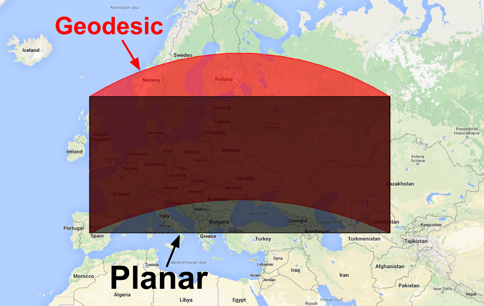
The parameter geodesic helps us to create geometries with straight edges (geodesic is by default TRUE). The figure below (extracted from here) shows the difference between the default geodesic polygon and the result of converting the polygon to a planar representation (geodesic = FALSE).

Note that the values of world_temp are in the range [0-1], to rescaled again the values to the real range we could use this simple trick:

min_lst <- landSurfaceTemperatureVis$min
max_lst <- landSurfaceTemperatureVis$max
world_temp[] <- scales::rescale(
  getValues(world_temp), c(min_lst, max_lst)
)

If you want to get the exact pixel value use ee_as_star or ee_as_raster instead of ee_as_thumbnail. Finally, we change the raster projection from longlat to Eckert IV (an equal-area pseudocylindrical map projection).

data("World") # Load world vector (available after load tmap)
world_temp_robin <- projectRaster(
  from = world_temp,
  crs = crs(World)
) %>% mask(World)

That’s all!. We are ready to create a static map using tmap!.

tm_shape(shp = world_temp_robin) +
  tm_raster(
    title = "LST (°C)",
    palette = cpt("grass_bcyr", n = 100),
    stretch.palette = FALSE,
    style = "cont"
  ) +
  tm_shape(shp = World) + 
  tm_borders(col = "black", lwd = 0.7) +
  tm_graticules(alpha=0.8, lwd = 0.5, labels.size = 0.5) +
  tm_layout() +
  tmap_style(style = "natural") +
  tm_layout(
    scale = .8,
    bg.color = "gray90",
    frame = FALSE,
    frame.lwd = NA,
    panel.label.bg.color = NA,
    attr.outside = TRUE,
    main.title.size = 0.8,
    main.title = "Global monthly mean LST from MODIS: January 2020",
    main.title.fontface = 2,
    main.title.position = 0.1,
    legend.title.size = 1,
    legend.title.fontface = 2,
    legend.text.size = 0.7,
    legend.frame = FALSE,
    legend.outside = TRUE,
    legend.position = c(0.10, 0.38),
    legend.bg.color = "white",
    legend.bg.alpha = 1
  ) +
  tm_credits(
    text = "Source: MOD11A1 - Terra Land Surface Temperature and Emissivity Daily Global 1km",
    size = 0.8,
    position = c(0.1,0)
  ) -> lst_tmap
tmap_save(lst_tmap, "lst_tmap.svg", width = 1865, height = 1165)

This is the end of this tutorial! the next week I will write a little about how to efficiently download large datasets using rgee.

The complete code is available here.