“Reinforcement learning”

Overview

In autonomous driving, the computer takes actions based on what it sees. It stops on a red light or makes a turn in a T junction. In a chess game, we make moves based on the chess pieces on the board. In reinforcement learning, we study the actions that maximize the total rewards. In stock trading, we evaluate our trading strategy to maximize the rewards which is the total return. Interestingly, rewards may be realized long after an action. Like in a chess game, we may make sacrifice moves to maximize the long term gain.

In reinforcement learning, we create a policy to determine what action to take in a specific state that can maximize the rewards.

In blackjack, the state of the game is the sum of your cards and the value of the face up card of the dealer. The actions are stick or hit. The policy is whether you stick or hit based on the value of your cards and the dealer’s face up card. The rewards are the total money you win or loss.

Known model

Iterative policy evaluation

Credit: (David Silver RL course)

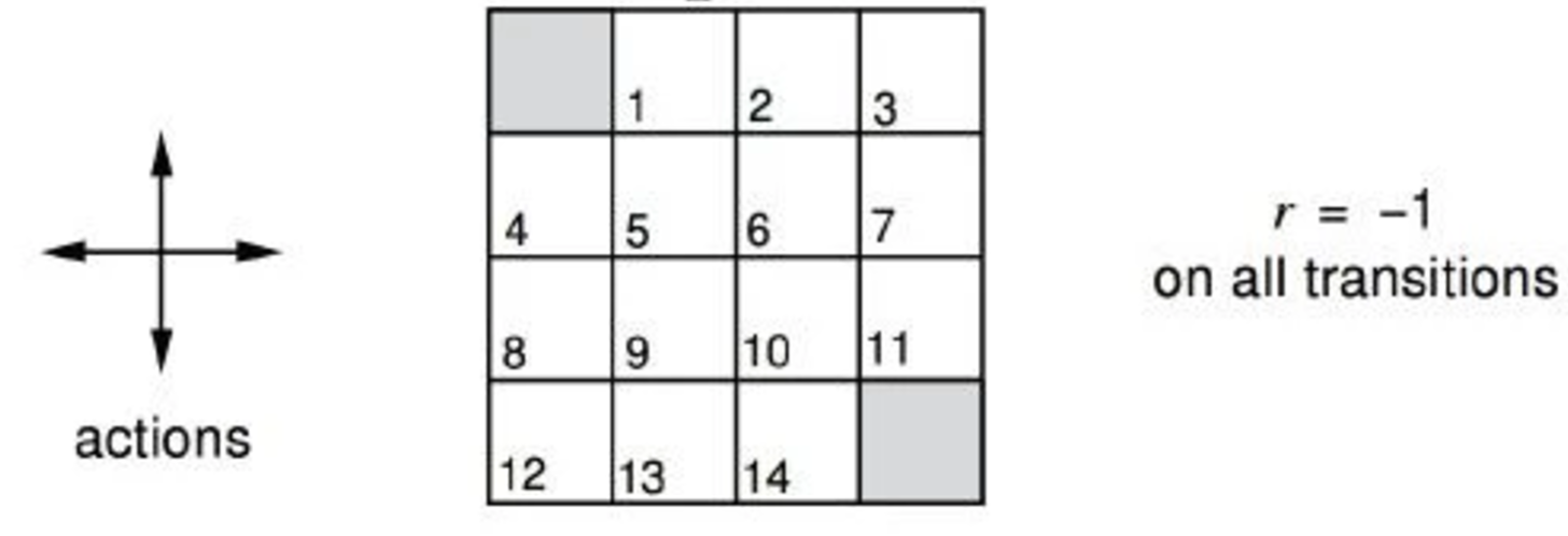
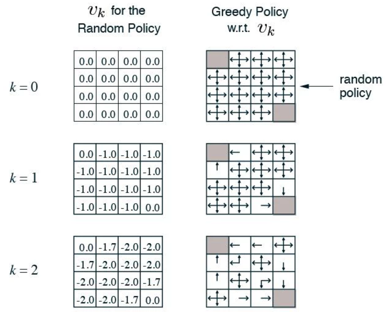
We divide a room into 16 grids and name each grid as above. At each time frame, we can move up, dow, left or right one step. However, we penalize each move by 1. i.e. we give a negative reward (-1) for every move. The game finishes when we reach the top left corner (grid 0) or the bottom right corner (grid 15). Obviously, with a negative reward, we are better off at grid 1 than grid 9 since grid 9 is further away from exits than grid 1. Here, we use a value function v(s) to measure how good to be at certain state. Let’s evaluate this value function with a random policy. i.e. at every grid, we have an equal chance of going up, down, left or right.

We initialize v(s) to be 0.

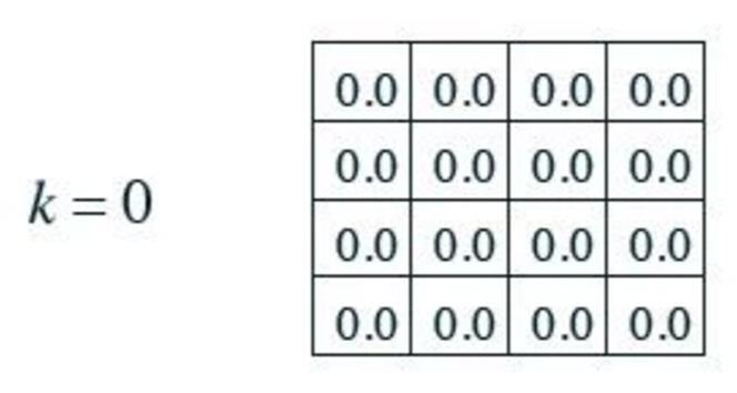
In our first iteration k=1, we compute a new value function for each state based on the next state after taking an action: We add the reward of each action to the value function of the next state. Then we compute the expected value function for all actions. For example, in grid 1, we can go down, left or right (not up) with a chance of 1/3 each. As defined, any action will have a reward of -1. When we move from grid 1 to grid 2, the reward is -1 and the v(s) for the next state grid2 is 0. The sum will be −1+0=−1. We repeat the calculation for grid 1 to grid 0 (moving left) and grid 1 to grid 5 (moving down) which are all equal to -1. Then we multiple each value with the corresponding chance (1/3) to find the expected value:

v(grid1)=1/3∗(−1+0)+1/3∗(−1+0)+1/3∗(−1+0)=−1

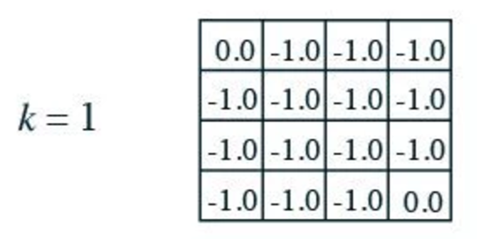
In the next iteration 2, the new value function for grid 1 is

v(grid1)=1/3∗(−1+0)+1/3∗(−1−1)+1/3∗(−1−1)=−1.666≈−1.7

and when we keep the iteration, the value function will converge to the final result for the random policy. For example, at grid 9, it will take an average of 20 steps to reach the exit point.

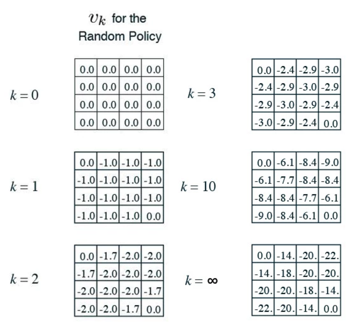
With the value function, we can easily create an optimal policy to exit the room. We just need to follow a path with the next highest value function:

In general, the value function vk+1(s) for state s at iteration k+1 is defined as:

Vk+1(s)=∑a∈Aπ(a|s)(Ras+γ∑s′∈SPass′Vk(s′))

Let us digest the equation further. The total estimated rewards (the right term) for taking action a at state s is:

Ras+γ∑s′∈SPass′Vk(s′)

Vk(s′) is the value function of the next state for taking a specific action. However, an action may transit the system to different states. So we define Pass′ as the probability of transfer from state s to s′ after taken action a. Hence, ∑s′∈SPass′Vk(s′) is the expected value function for all possible next states after action a at state s. γ (0<γ<=1) gives an option to discount future rewards. For rewards further away from present, we may gradually discount it because of its un-certainty or to favor a more stable mathematical solution. For γ<1, we pay less weight to future rewards than present. Ras is the reward given of taking action a at state s. So the equation above is the total estimated rewards for taking action a at state s.

In our example, each action only lead to a single state and hence there is only one output state and Pass′=1. The new estimated total reward is simplify to:

Ras+γVk(s′)

This simplified equation is the corner stone in understanding and estimating total rewards.

π is our policy and π(a|s) is the probability for taking action a given the state s. So the whole equation for Vk+1(s) is the expected value functions for taken all possible actions for a state.

In our example, with γ=1 (no discount on future reward), the equation is simplify to:

Vk+1(s)=∑a∈Aπ(a|s)(Ras+Vk(s′))

V2(grid1)=∑a∈Aπ(a|s)(−1+vk(s′))=1/3∗(−1+0)+1/3∗(−1−1)+1/3∗(−1−1)≈−1.7

which s′ is the next state (grid 5, grid 0, grid 2) for action down, left, right respectively.

Policy iteration

In policy iteration, our goal is to find the optimal policy rather then the value function of a particular policy. In last section, we hold the policy constant throughout the calculation. In policy iteration, we do not keep the policy constant. In fact, we update to a new policy in every iteration based on the value function:

Credit: (David Silver RL course)

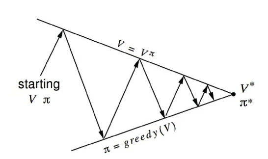
At each iteration, we start with the value function Vk and policy π. Then we compute the value function Vk+1 for this iteration. Then based on the new value function, we replace the policy by a new greedy policy based on Vk+1

π=greedy(Vk+1)

At the right, we start with a random policy which updated at every iteration. As shown below, after 2 iterations, we can find the optimal policy to reach the exit the fastest.

Model free

In the example above, we assume the reward and the state transition is well known. In reality, it is not often true in particular robotics. The chess game model is well known. But some games like the Atari ping-pong, the model is not known precisely by the gamer. In the Go game, the model is well known but the state space is so huge that it is computationally impossible to calculate the value function using the methods above. With a model free example, we need to execute an action in the real environment or a simulator to find out the reward and the next transition state for that action.

Model free RL executes actions to observe rewards and state changes to calculate value functions or policy.

Monte-Carlo learning

We turn to sampling hoping that after playing enough games, we find the value function empirically. In Monte-Carlo, we start with a particular state and keep continue playing until the end of game.

For example, we have one episode with the following state, action, reward sequence. S1,A1,R2,...,St,At,Rt+1,...

At the end of the game, we find the total reward Gt (total rewards from St to the end) by adding rewards from Rt+1 to the end of the game. We update the value function by adding a small portion of the difference between new estimate Gt and the current value V(St) back to itself. This approach creates a running mean from a stream of estimates. With many more episodes, V(St) will converge to the true value.

V(St)=V(St)+α(Gt−V(St))

Temporal-difference learning (TD)

Let’s say we want to find the average driving time from San Francisco to L.A. We first estimate that the trip will take 6 hours and we have 6 check points suppose to be 1 hour apart. We update the estimation of SF to LA after the first check point. For example, it takes 1.5 hour to reach the first check point Dublin. So the difference from the estimation is (1.5+5)−6=0.5. We add a small portion of the difference back to the estimation. In the next check point, we update the estimation time from Dublin to LA.

In temporal-difference (TD), we look ahead 1 step to estimate a new total reward by adding the action reward to the value function of the next state (similar to 1.5+1 above):

V′(St)=Rt+1+γV(St+1)

We compute the difference of V(St) and V′(St). Then we add a portion of the difference back to V(St).

δ=Rt+1+γV(St+1)−V(St)V(St)=V(St)+αδ

For a single episode, S1,A1,R2,...,St,At,Rt+1,....,Slast,Alast,, we update V(S1) to V(Slast) each with a one step look ahead as above. After repeating many episodes, we expect V to converge to a good estimate.

TD(λ)

In TD, we use a 1 step look ahead: use the reward Rt+1 to update Vt.

G1t=Rt+1+γV(St+1)V(St)=V(St)+α(G1t−V(St))

We can have a 2 step look ahead: Take 2 actions and use the next 2 rewards to compute the difference.

G2t=Rt+1+γ(Rt+2+γV(St+2))V(St)=V(St)+α(G2t−V(St))

In fact, we can has n-step look ahead with n approaches infinity. To update V(St), we can use the average of all these look ahead.

V(St)=V(St)+α1N(δ1(St)+...+δN(St)))

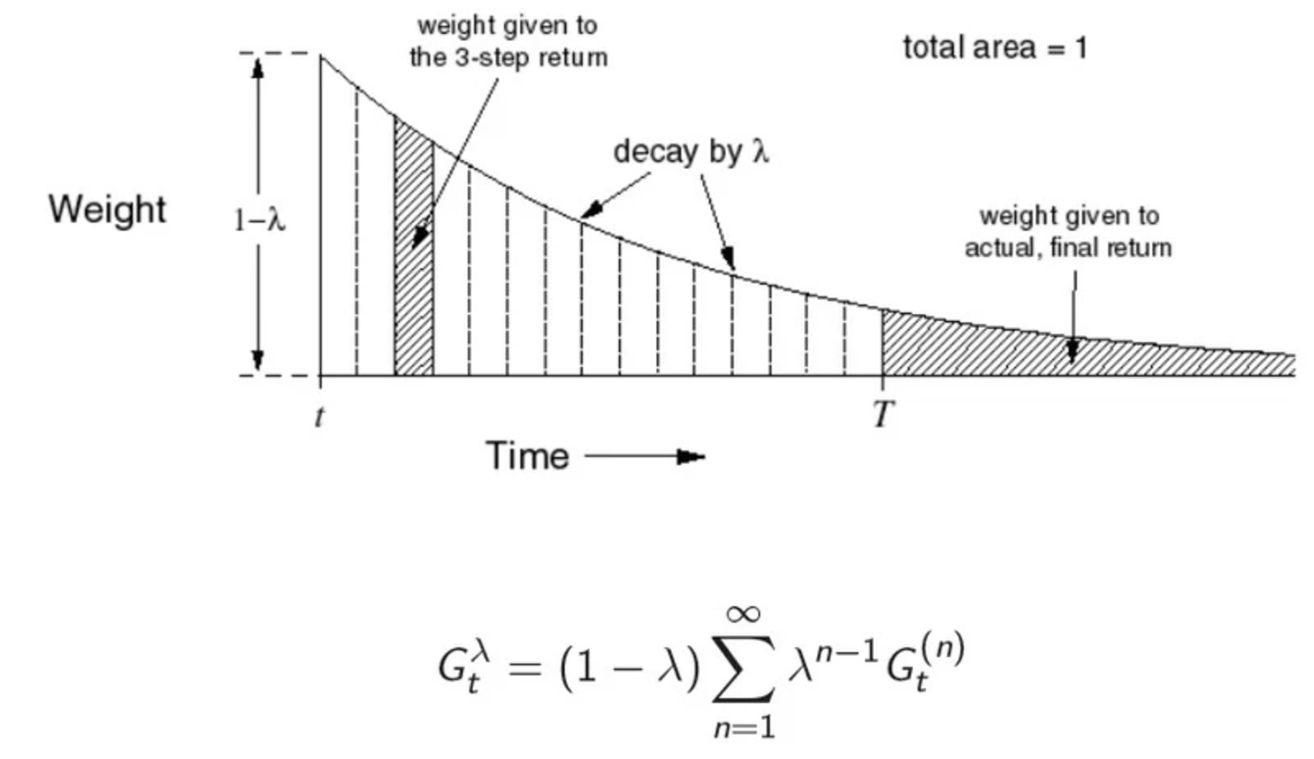
In TD(λ), however, we don’t take the average. The weight drops as k increase in Gkt (in kth steps look ahead). The weight we use is:

Gt(λ)=(1−λ)∞∑n=1λn−1Gnt

The value function is:

V(St)=V(St)+α(Gt(λ)−V(St))

When λ=0, this is TD and when λ=1, it is Monte-carlo. The following demonstrates how the weight decrease for each kth-step.

Source: David Silver RL class.

Eligibility traces & backward view TD(λ)

We do not compute TD(λ) directly in practice. Mathematically, TD(λ) is the same as Eligibility traces.

First we compute the eligibility traces:

E0(s)=0Et(s)=γλEt−1(s)+1(St=s)

When we visit a state s, we add 1 to Et(s) which record the current trace level for state s at time t. But at the same time, we decay the trace as time pass. In the diagram below, the vertical bar at the bottom indicates when state s is visited. We can see the trace value jumps up by approximately 1 unit. But it the same time, we gradually decay the trace by γλEt−1(s) Hence we see the trace decay when there is not new visit. The intuition is to update the estimate more aggressive for states visited closer to when a reward is granted.

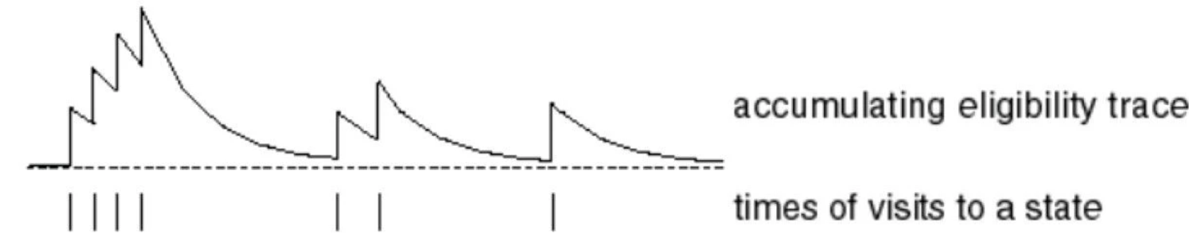
Source: David Silver RL course.

We first compute the differences in the estimates. Then we use the eligibility traces as weight of how to update the previous visited states in this episode.

δt=Rt+1+γV(St+1)−V(St)V(s)=V(s)+αδtEt(s)

Model free control

With a model, we optimize policy by taking an action using the greedy algorithm. i.e. in each iteration, we look at the neighboring states and determines which path gives us the best total rewards. With a model, we can derive the action that take us to that state. Without a model, V(s) is not enough to tell which action to take to get to the next best state. Now instead of estimate value function for a state v(s), we estimate the action value function for a state and an action Q(s,a). This value tells us how good to take action a at state s. This value will help us to pick which action to execute during the sampling.

Monte-Carlo

The corresponding equation to update Q with Monte-Carlo is similar to that for V(s)

Q(St,At)=Q(St,At)+α(Gt−Q(St,At))

which Gt is the total rewards after taking the action At

However, we do not use greedy algorithm to select action within each episode. Similar to all sampling algorithm, we do not want outliner samples to stop us from exploring the sample action. A greedy algorithm may pre-mature stop us for actions that look bad in a few sample but in general performs very well. But when we process more and more episodes, we will have more exploitation for known good actions rather than exploring more less promising actions to avoid outliner samples.

To sample the kth episode, S1,A1,R2,...,St,At,Rt+1,....,Slast,Alast,, we use a ε-greedy algorithm below to pick which action to sample next. For example, at S1, we use it to compute the policy π(a|s1). Then we sample an action as A1 based on this distribution.

ε=1/kπ(a|s)={ε/m+1−ε,if a∗=argmaxaQ(s,a)ε/m,otherwise

As k increases, the policy distribution will favor action with higher Q value.

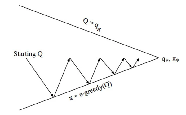
Eventually, similar to the previous policy iteration, argmaxaQ(s,a) will be the optimal policy.

Sarsa

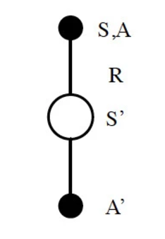
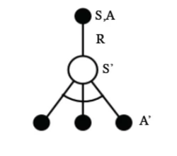
Sarsa is the corresponding TD method for estimate Q without a model. At state S, we sample an action based on Q(s,a) using ε-greedy. We received an reward and transit to s′. Once again, we sample another action a′ using ε-greedy and use the Q(s′,a′) to update Q(s,a).

Q(S,A)=Q(S,A)+α(R+γQ(S′,A′)−Q(S,A))

Here is the algorithm

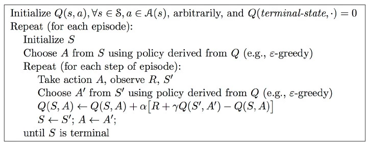
Source: David Silver RL course

Sarsa(λ)

Because its close similarity with TD(λ), we will just show the equations.

To update the Q value:

Qt(λ)=(1−λ)∞∑n=1λn−1QntQ(St,At)=Q(St,At)+α(Qt(λ)−Q(St,At))

Sarsa with eligibility traces

Equation for the eligibility trace:

E0(s,a)=0Et(s,a)=γλEt−1(s,a)+1(St=s,At=a)

Update the Q:

δt=Rt+1+γQ(St+1,At+1)−Q(St,At)Q(s,a)=Q(s,a)+αδtEt(s,a)

Here is the algorithm

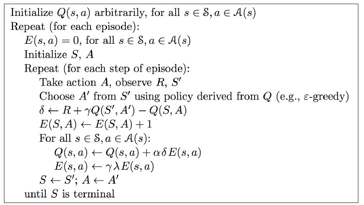
Source: David Silver RL course

Q-learning (Sarsa Max)

In Sarsa, we use

Q(S,A)=Q(S,A)+α(R+γQ(S′,A′)−Q(S,A))

Both A and A′ are sampled using ε-greedy algorithm. However, in Q-learning, a is picked by ε-greedy algorithm but a′ is picked by

argmaxa′Q(s′,a′)

i.e. select the second action with the highest action value function Q(s′,a′)

Credit: David Silver RL course

The formular will therefore change to:

Q(S,A)=Q(S,A)+α(R+γargmaxa′Q(s′,a′)−Q(S,A))

The ε-greedy algorithm explores states with high un-certainty in earlier episode. But it also lead the training to very bad state more frequently. Q-learning using greedy algorithm in their second pick. With the combination of ε-greedy algorithm, at least in the empirical data, it helps the training to avoid some very disaster states. It therefore trains the model better.

Here is the algorithm

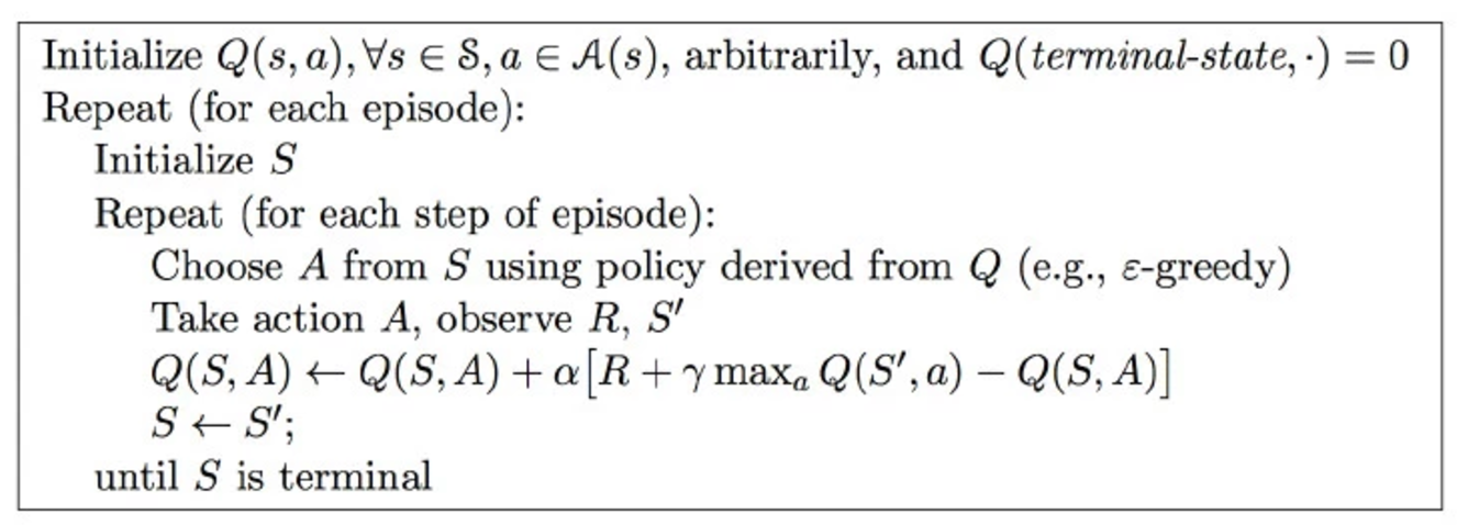
Credit: David Silver RL course

Value function estimator

In previous sections, we focus on computing V or Q accurately through sampling experience. If the system has a very large space for the states, we need a lot of computations and memory to compute so many function values. Instead, we turn to deep learning networks to approximate them. i.e. we build a deep network to estimate V or Q.

The cost function of a deep network for V is defined as the mean square error between the network estimation and sampling experience:

J(w)=Eπ[(vπ(s)−ˆv(S,w))2]

which ˆv(S,w) is the output value from the deep network and vπ(s) is the calculated value using our sampling episodes. We then backpropagate the gradient of the lost function to optimize the trainable parameters of the deep network.

∇wJ(w)=2⋅(vπ(s)−ˆv(S,w))∇wˆv(S,w)△w=−12α∇wJ(w)=α(vπ(s)−ˆv(S,w))∇wˆv(S,w)

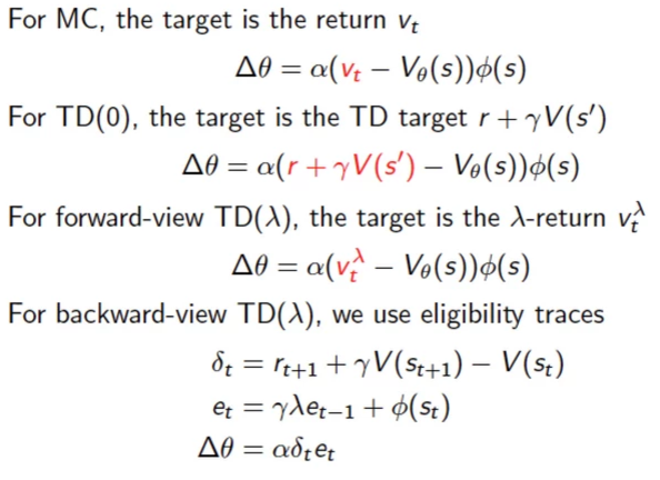
We can using different methods described before to compute vπ(s) through sampling. For example, we can work with Monte-Carlo, TD or TD(λ) on V to optimize the deep network.

△w=α(Gt−ˆv(St,w))∇wˆv(St,w)Monte-Carlo△w=α(Rt+1+γˆv(St+1,w)−ˆv(St,w))∇wˆv(St,w)TD△w=α(Gt(λ)−ˆv(St,w))∇wˆv(St,w)TD(λ)δt=Rt+1+γˆv(St+1,w)−ˆv(St,w)Eligibility traceEt=γλEt−1+1(St=s)△w=αδtEt

Alernatively, we can use Monte-Carlo, Sarsa, Sarsa(λ) or Q-learning on Q.

△w=α(Gt−ˆq(St,At,w))∇wˆq(St,At,w)Monte-Carlo△w=α(Rt+1+γˆq(St+1,At+1,w)−ˆq(St,At,w))∇wˆq(St,At,w)Sarsa△w=α(qt(λ)−ˆq(St,At,w))∇wˆq(St,At,w)Sarsa(λ)△w=α(Rt+1+γ⋅argmaxa′ˆq(St+1,a′,w)−ˆq(St,At,w))∇wˆq(St,At,w)Q-learningδt=Rt+1+γˆa(St+1,At+1,w)−ˆq(St,At,w)Eligibility traceEt=γλEt−1+1(St=s,At=a)△w=αδtEt

We can updates w immediately at each step of an episode. However, this may de-stabilize our solution. Instead, we accumulate the gradient changes and change the network parameter only after batches of episodes.

Deep Q-learning network (DQN)

DQN is less important comparing to the Policy gradient in the next section. Hence, we will not explain DQN in details. But it is helpful to understand how to apply deep network in approximating function values or policy.

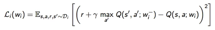
DQN uses deep learning network to approximate the action value function and use Q-learning target in the gradient descent. The gradient of the lost function is defined as:

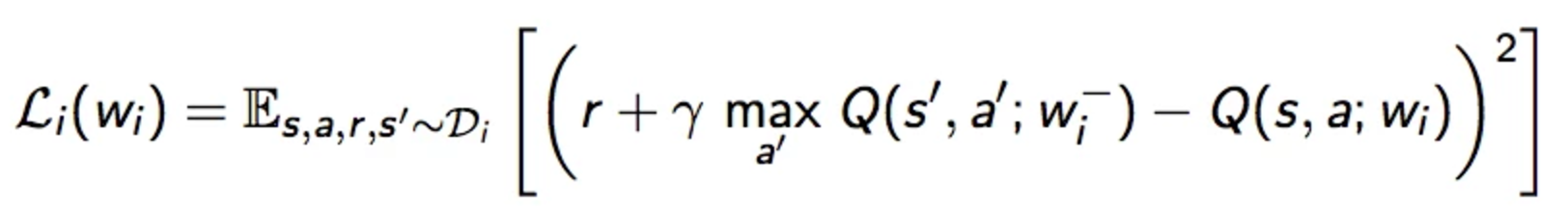
Gradient of the lost function:

DQN uses ε-greedy algorithm to select an action at randomly or based on argmaxaQ(st,a,w) for the state st. Here, we use a deep network to compute Q(st,a,w) for the best action. We store the sequence (st,at,rt+1,st+1) into a replay memory D. We sample batches of sequence from the replay memory to train the network. (experience replay) We compute the Q-learning target with values from the sampled experience and the Q values estimated by the deep network. We apply gradient descent to optimize the deep network.

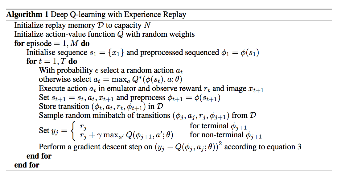
Source: DeepMind Eq 3 is the gradient of the lost function.

We are selecting actions using the deep network parameterize by w while we are simultaneously optimizing those w with gradient descent. However, this is mathematically less stable. DQN uses a fixed Q-target which the action selection is based on the older copy w− which is updated at the end of the batches of episodes.

Policy Gradient

In previous sections, we look at many different states and compute how good they are. Then we formulate a policy to reach those states. Alternatively, we can start with a policy and improve it based on the observation. Previous algorithms focus on finding the value functions V or Q and derive the optimal policy from it. Some algorithms recompute the value functions of the whole state space at each iteration. Unfortunately, for problems with a large state space, this is not efficient. The model free control improves this by using ε-greedy algorithm to reduce the amount of state space to search. It focuses on actions either not been explore much or that have high Q value.

Alternatively, instead of focus on the value function first. We can focus on the policy first. Policy gradient focuses on finding the optimal policy πθ(a|s) given a state s. We use deep network to predict the best action for a specific state. The principle is pretty simple. We use the deep network to tell us what action to take for a specific state. We observe the result. If it is good, we tune the network to be more confidence in making such suggestion. If it is bad, we train our network to make some other prediction.

A shooting sequence can break down into many frames. With policy gradient, the deep network determines what is the best action to take at each frame to maximize the success.

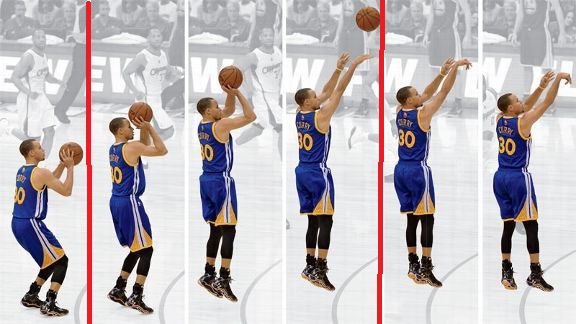
Source ESPN

Technically, we adjust the deep network to make policy that yields better total rewards. Through Monte-Carlo or TD(λ), we can estimate how good to take a specific action ai at a particular state s. If it is good, we backpropagate the gradient to make changes to θ such that the score predicted by the deep network πθ(ai|s) is high.

Total rewards

Let’s calculate the total rewards J(θ) of a single step system. i.e. we sample a state s from a state probability distribution d(s) from this system, take an action a, get a reward r=Rs,a and then immediately terminate. The total rewards will be:

J(θ)=Eπθ(r)=∑s∈Sd(s)∑a∈Aπθ(s,a)Rs,a∇θJ(θ)=∑s∈Sd(s)∑a∈A∇θπθ(s,a)Rs,a=∑s∈Sd(s)∑a∈Aπθ(s,a)∇θπθ(s,a)πθ(s,a)Rs,a=∑s∈Sd(s)∑a∈Aπθ(s,a)(∇θlogπθ(s,a))Rs,a=Eπθ((∇θlogπθ(s,a))r)=Eπθ((∇θscorea)r)

Our objective is to maximize the total rewards J(θ). i.e. build a deep network that makes good action predictions with the highest total rewards. To do that, we compute the gradient of the cost function so we can optimize the deep network. The term logπθ(s,a) should be familiar in deep learning. This is the log of a probability. i.e. the logit value in a deep network. Usually, that is the score before the softmax function. Our solution ∇θJ(θ) depends on Rs,a and scorea. Rs,a measures how good is the action and scorea on how confidence the deep network about the action. When Rs,a is high, we backpropagate the signal to change θ in the deep network to boost scorea. i.e. we encourage the network to predict actions that give good total rewards.

Without proofing, the equivalent equations for multiple steps system is:

∇θJ(θ)=Eπθ((∇θlogπθ(s,a))Qπθ(s,a))=Eπθ((∇θscorea)Qπθ(s,a))

And we can use the gradient to optimize the deep network.

Policy Gradient using Monte-Carlo

We can sample Qπθ(s,a) using Monte-Carlo and use the lost function gradient to train the network. The algorithm is:

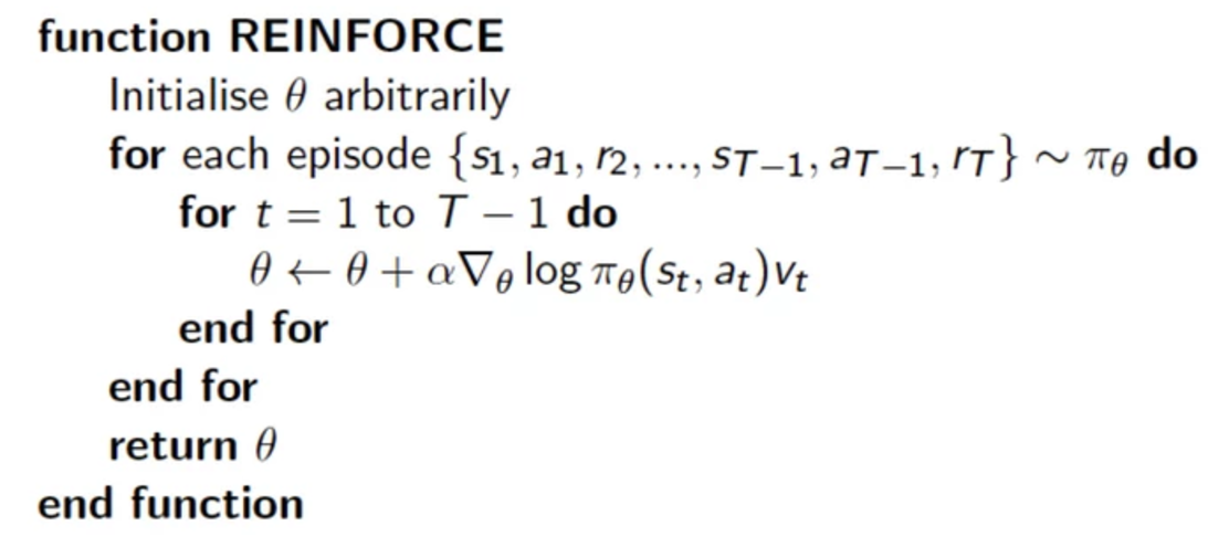
Source David Silver Course

Advantage function

Qπθ(s,a) is high variance with Monte-Carlo. One value calculated from one sampling path in Monte-Carlo can have very different value in another sampling path. For example, just make a change in one move in chess can produce total different result. We try to reduce the variance by subtracting it with a baseline value V(s). We can proof that it produces the same solution for ∇θJ(θ) even we replace Qπθ(s,a) with Qπθ(s,a)−Vπθ(s)

Let’s proof that the following term is equal to 0 first:

Eπθ((∇θlogπθ(s,a))B(S))=∑s∈Sd(s)∑a∈A∇θπθ(s,a)B(s)=∑s∈Sd(s)B(s)∇θ∑a∈Aπθ(s,a)=∑s∈Sd(s)B(s)∇θ1=0

Replace Qπθ(s,a) with Qπθ(s,a)−Vπθ(s) will produce the same solution for θ:

Eπθ((∇θscorea)(Qπθ(s,a)−Vπθ(s)))=Eπθ((∇θscorea)(Qπθ(s,a)))−Eπθ((∇θscorea)Vπθ(s))=Eπθ((∇θscorea)(Qπθ(s,a)))=∇θJ(θ)

We call this the advantage function:

Aπθ(s,a)=Qπθ(s,a)−Vπθ(s)

We use it to replace Qπθ(s,a) in training the deep network.

Here, we can proof that we can use TD(λ) method as the advantage function.

δπθ=r+γVπθ(s′)−Vπθ(s)Eπθ(δπθ|s,a)=Eπθ(r+γVπθ(s′))−Vπθ(s)=Qπθ(s,a)−Vπθ(s,a)=Aπθ(s,a)

Here are the different methods to train θ of the deep network.

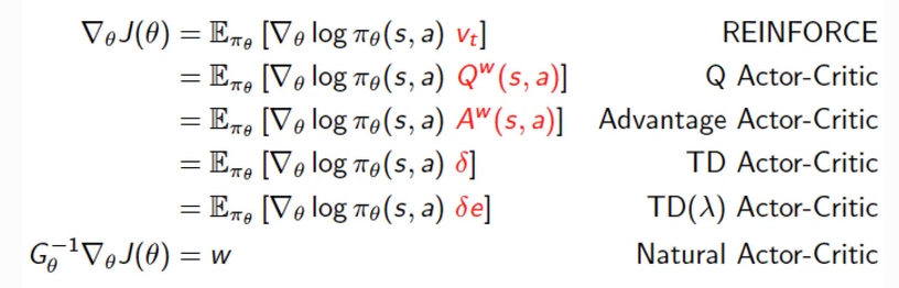
And some example if score is simply computed with a linear regression:

score=ϕ(s)Tθ

∇θlogπ(s)=∇θscore(s)=∇θϕ(s)Tθ=ϕ(s)

Source David Silver Course

Reinforcement learning for Atari pong game

The code in this section is based on Andrej Karpathy blog.

Let’s solve the Atari Pong game using reinforcement learning.

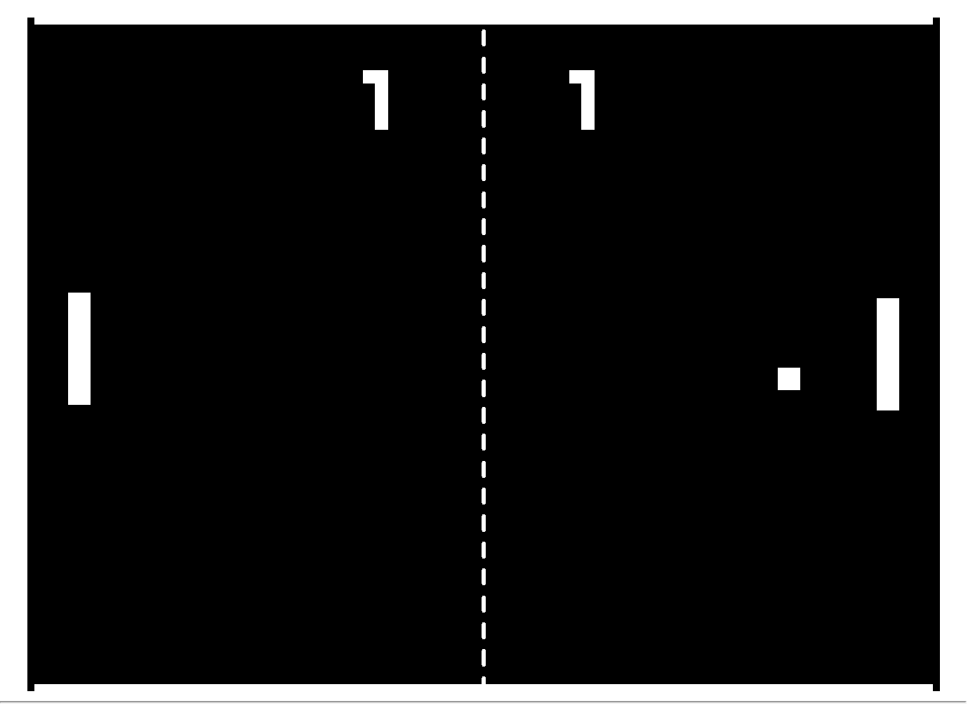
We are using the OpenAI gym to create a simulation environment for the Pong game. This simulation environment will feed us frame images of size 210x160x3 as input to the program. We get a reward of 1 when we win a game and -1 when we lost one. The objective of the code is to develop an optimal policy for moving the paddle up or down by observing the image frame.

We are going to use Policy gradient to train a network to predict those actions based on the image frames that feed into the system.

State of Atari pong game

We will initialize the OpenAI Gym’s Pong game to give us the first image frame of the game. After that, whenever we take an action (moving the padding up or down), the Pong game will feed us an updated image frame. Whenever we receive an image frame, we will preprocess it including cropping and background removing. The preprocess generates a 80x80 black and white image which we will flatten it into an array of 6400 values of either 0 or 1. In order to capture the motion, we will subtract it with the previous pre-processed frame. So the final array contains the difference of the current frame and the previous frame to capture motion. This (6400, ) array will be the input to our network.

Here we initialize the OpenAI Gym Atari game and reset the game to get the first image frame

env = gym.make("Pong-v0")
observation = env.reset() # One image frame of the game. shape: (210, 160, 3)

We preprocess each frame and find the difference between the current frame and the last frame. The result is an array of 6400 values (80x80) containing either 0, 1 or -1. x will be forward feed into our model.

# Preprocess the observation.
# Crop it to 80x80, flatten it to 6400. Set background pixels to 0. Otherwise set the pixel to 1.
cur_x = prepro(observation)

# Compute the difference of current frame and the last frame. This captures motion.
x = cur_x - prev_x if prev_x is not None else np.zeros(D)
prev_x = cur_x

Model

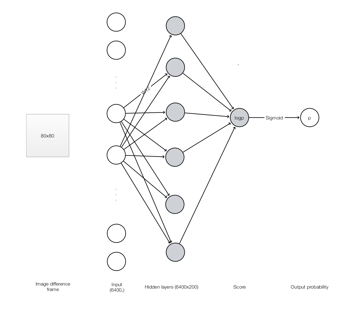
The model will take an array of 6400 values. It forward feed the input to a fully connected hidden layer of 200 nodes with output passed through a ReLU. We then have an output layer to map those 200 nodes to a single score value (logp). Afterwards, we use a sigmoid function to convert the score to a probability (p) for the chance of taking the action #2.

Here is the forward feed code include 1 hidden layer follow with another output layer

def policy_forward(x):
    """
        x is the input feature of shape (6400,)
        model['w1'] shape (200, 6400)
        model0'w2'] shape (200,)
        return p (probability): scalar
               h (hiddend states of 1st layer): (200,)
    """
    h = np.dot(model['W1'], x) # The hidden layer
    h[h < 0] = 0               # ReLU nonlinearity
    logp = np.dot(model['W2'], h) # Output a single score
    p = sigmoid(logp)             # Use sigmoid to convert to a probability
    return p, h                   # return probability of taking action 2, and hidden state

The forward feed code return a probability (p) which is our policy for action #2 πθ(action #2|x). We sample an action based on this probability. We then call the Pong game with our next action, and the game will return the next image frame and the reward. We will also record the rewards in every step.

aprob, h = policy_forward(x)
action = 2 if np.random.uniform() < aprob else 3  # roll the dice!

observation, reward, done, info = env.step(action)
drs.append(reward)  # record reward (has to be done after we call step() to get reward for previous action)

The game returns 1 (variable reward) if you win, -1 if you loss and 0 otherwise. In our first game, we receive 0 for the first 83 steps and then -1. We loss the first game. Here we record our reward at each step as:

(0,0,0,...,−1)

Recall that the total rewards at each step is computed as following:

Gt=Rt+1+γV(St+1)

If γ=1, G=(−1,−1,−1,....−1). However, we apply γ=0.99. i.e. We consider the reward is less significant if it is further way from when the reward is granted. We apply the adjustment and here is the total rewards of our first game (Received -1 at step 83.):

G=(−0.434,−0.44,−0.443,−0.448,...,−0.98,−0.99,−1.0)

Backpropagation

Here we initialize the gradient needed for the backpropagation.

gradient={(1−p)⋅Gt,action=2(−p)⋅Gt,otherwise

Initial gradient is proportional to the total reward Gt

aprob, h = policy_forward(x)
action = 2 if np.random.uniform() < aprob else 3

y = 1 if action == 2 else 0
dlogps.append(y - aprob)

Each game is “done” when either player win 21 games. Once it is done, we backpropagate the gradient to train the network.

observation, reward, done, info = env.step(action)
...

if done:  # Game is done when one side reaches 21 points
    # compute the discounted reward backwards through time
    epr = np.vstack(drs)       
    discounted_epr = discount_rewards(epr)

    epdlogp = np.vstack(dlogps)
    epdlogp *= discounted_epr

    grad = policy_backward(eph, epdlogp)

With backpropagation, we compute the gradient for each trainable parameters.

def policy_backward(eph, epdlogp):
    """
        backward pass. (eph is array of intermediate hidden states)
    """
    dW2 = np.dot(eph.T, epdlogp).ravel()
    dh = np.outer(epdlogp, model['W2'])
    dh[eph <= 0] = 0                       # backpro prelu
    dW1 = np.dot(dh.T, epx)
    return {'W1': dW1, 'W2': dW2}

Training

The rest of the training is no different from training a deep network. Here we accumulate all the gradients and make change to trainable parameters every 10 batches of games using the RMSProp (each game lasts until one player score 21 points).

# Add all the gradient for steps in an episode
for k in model:
     grad_buffer[k] += grad[k]  # accumulate grad over batch; grad_buffer['w1']:(200, 6400), grad_buffer['w1']:(200,)

# perform rmsprop parameter update every batch_size episodes
if episode_number % batch_size == 0:
   for k, v in model.iteritems():
      g = grad_buffer[k]  # gradient
      rmsprop_cache[k] = decay_rate * rmsprop_cache[k] + (1 - decay_rate) * g ** 2
      model[k] += learning_rate * g / (np.sqrt(rmsprop_cache[k]) + 1e-5)
      grad_buffer[k] = np.zeros_like(v)  # reset batch gradient buffer

The source code can be find here.

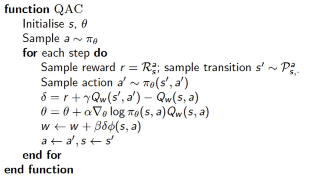
Policy gradient using Actor and Critic

Policy gradient needs to know how good is an action with a specific state. Qπθ(s,a)

∇θJ(θ)=Eπθ((∇θscorea)Qπθ(s,a))

In previous section, we use Monte-Carlo, TD, etc… to sample the value. However, we actually can have a second deep network to estimate this value. So we have one actor deep network to predict the policy and an critic deep network to predict the action value function. So critics learns how to evaluate how good is Q(s,a) and the actor deep network learns how to make good policy prediction πθ(a|s).

This is the algorithm:

Learning and planning

In previous sections, we sample states and take actions to be played in the real world or a simulator to collect information on rewards and transition states. (learning) Even we start with a modeless problem, we can use the observed data to peek into the model to have our algorithms to work better (planning).

Consider a system with state A and B. We use Monte-Carlo to build experience with the system. The left side is the state we sampled with the corresponding rewards. For example, we start with state A, the system gives us 0 reward when we transition to B. We transit to a terminate state and again with 0 reward. We play 7 more episodes which all starts at state B. Using Monte-Carlo, v(A)=0 and v(B)=0.75.

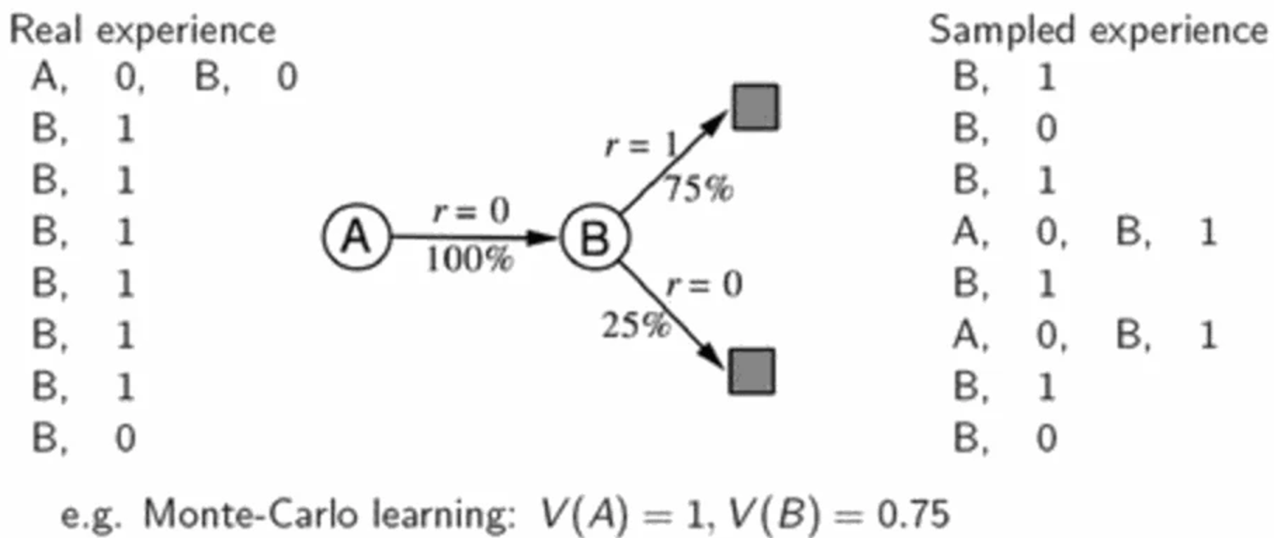
From the experience, we can build a model like the middle. Based on this model, we can sample data as in the right hand side. With the sampled experience, v(A)=1 and v(B)=0.75. The new v(A)=1 is closer to the real v(a) than one with just the real experience. So this kind of experience sampling and replay usually gives us better estimation of the value function.

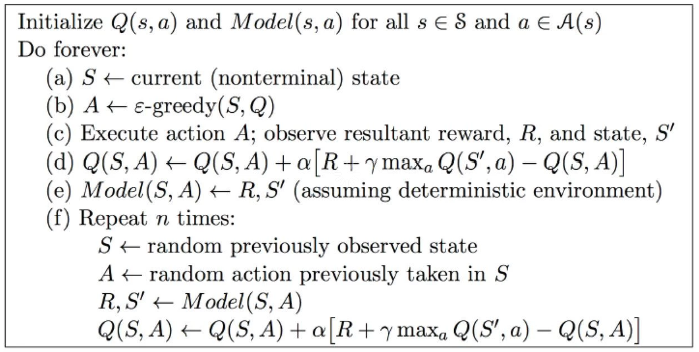
Here is the Dyna algorithm than use learning and planning to have a better estimate for Q.

Credits

The theory on Reinforcement learning is based on the David Silver class.

The code for Atari Pong game is based on Andrej Karpathy blog.