

“DRAW - Deep recurrent attentive writer”
source link: https://jhui.github.io/2017/04/30/DRAW-Deep-recurrent-attentive-writer/
Go to the source link to view the article. You can view the picture content, updated content and better typesetting reading experience. If the link is broken, please click the button below to view the snapshot at that time.

First, a quick review on variation autoencoder
In a previous article, we describe ways to generate images using a generative model like variational autoencoders (VAE). For example, we train a VAE to generate handwritten-like digits:
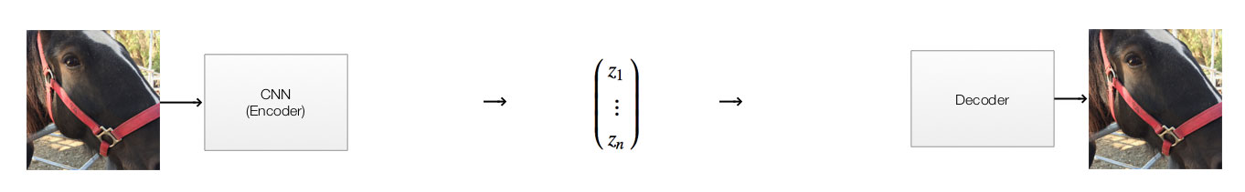
In an autoencoder, we encode an image with a lower dimensional vector. For example, we can encode a 256x256x3 RGB image with a 100-D latent vector z (x1,x2,...x100)(x1,x2,...x100). We reduce the dimension from 197K to 100. We later regenerate the images from the latent vectors. We train the network to minimize the difference between the original and the generated images. By significantly reducing the dimension, the network is forced to retain the important features so it can regenerate the original images back as close as possible.
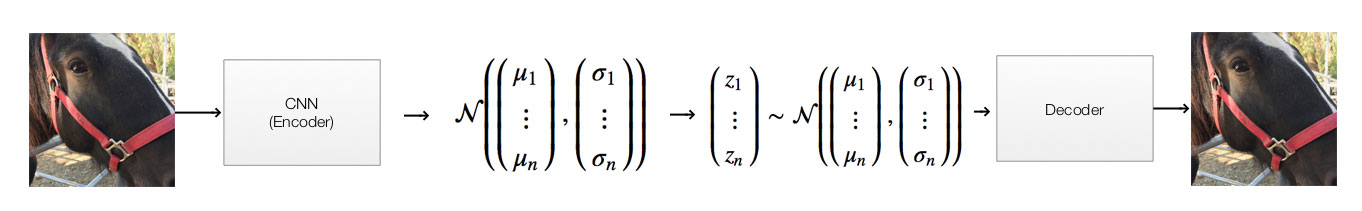
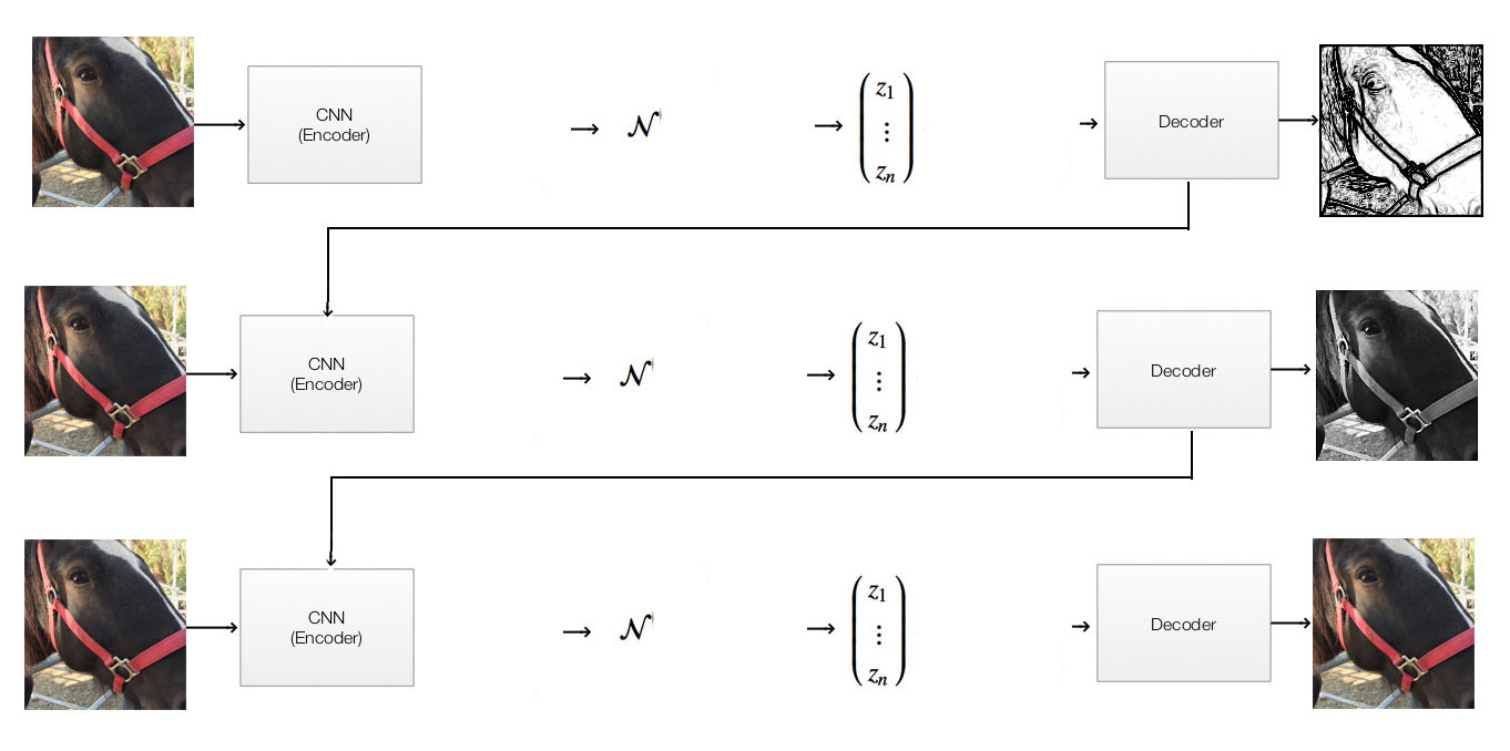
For a variation autoencoder, we replace the middle part with 2 separate steps. VAE does not generate the latent vector directly. It generates 100 Gaussian distributions each represented by a mean (μi)(μi) and a standard deviation (σi)(σi). Then it samples a latent vector, say (0.1, 0.03, …, -0.01), from these distributions. For example, if element xixi of the latent vector has μi=0.1μi=0.1 and σi=0.5σi=0.5. We randomly select xixi with probability based on this Gaussian distribution:
Real images does not take on all possible values. Constraints exist in real images. We can train our network more effective if we apply proper constraints. In a variation autoencoder, we penalize the network if the distribution of the latent vector zz made by the encoder is different from a normal gaussian distribution (i.e.., μ=0,σ=1μ=0,σ=1). Without going into the details, this penalty acts as a regularization cost to force the network not to memorize the training data (overfitting). It forces the network to encode as much features as possible with similar images having similar latent vectors.
In non-supervising learning, like clustering, one key objective is to group similar datapoints together by encoding them with similar encoding values.
Intuition for DRAW - Deep recurrent attentive writer
Google Deepmind’s DRAW (Deep recurrent attentive writer) further combines the variation autoencoder with LSTM and attention. Reducing the dimension in representing an image, we force the encoder to learn the image features. But doing the whole process in one single step can be hard. When people draw, people break it down into multiple steps.
The intuition of DRAW is to repeat the decode/encode step using a LSTM.
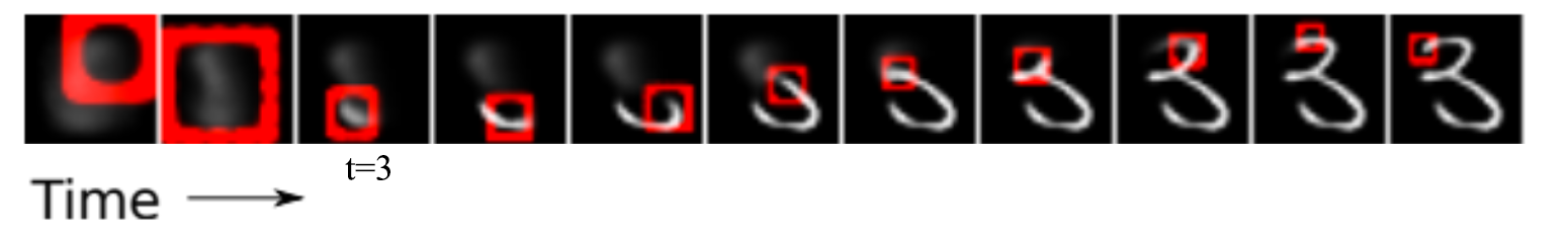
In each time step, we generate images closer and closer to the original image:
Attention
In each time iteration, instead of the whole image, we just focus on a smaller area. For example, at t=3t=3 below, the attention area (the red rectangle) is narrow down to the bottom left area of a “3”. At that moment, DRAW focuses in drawing this area only. As time moves on, you can tell the program is stroking a “3” in the reverse direction which we usually draw a “3”.
LSTM implementation
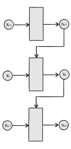
Recall a LSTM cell takes 2 input (hidden state at the previous time step and the current input):
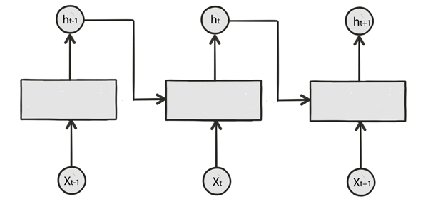
We are going to modify a single step model to a LSTM model for DRAW:
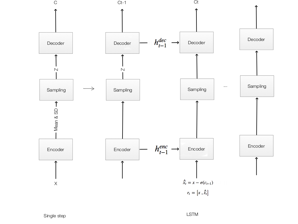
At each time step, we are going to comput the following equations:
Encoding:
Sampling:
Decoding:
Output:
Encoder
The encoder have 4 inputs:
- The original image xx and the residual image xt^=x−σ(ct−1)xt^=x−σ(ct−1).
- The hidden states of the encoder and decoder henct−1,hdect−1ht−1enc,ht−1dec from the previous timestep.
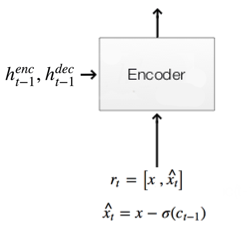
Original image & residual image:
c_prev = tf.zeros((self.N, 784)) if t == 0 else self.ct[t - 1]  # (N, 784)
x_hat = x - tf.sigmoid(c_prev)  # residual: (N, 784)
r = tf.concat([x,x_hat], 1)
Using LSTM and 2 FC for Encoder:
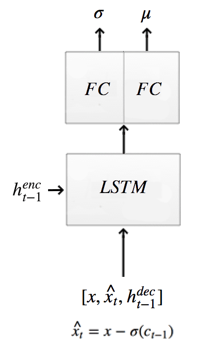
The encoder computes the hidden states and the Gaussian distribution of the latent variable zz:
self.mu[t], self.logsigma[t], self.sigma[t], enc_state = self.encode(enc_state,
                                                         tf.concat([r, h_dec_prev], 1))
def encode(self, prev_state, image):
   # update the RNN with image
   with tf.variable_scope("encoder", reuse=self.share_parameters):
       hidden_layer, next_state = self.lstm_enc(image, prev_state)

   # map the RNN hidden state to latent variables
   # Generate the means using a FC layer
   with tf.variable_scope("mu", reuse=self.share_parameters):
       mu = dense(hidden_layer, self.n_hidden, self.n_z)

   # Generate the sigma using a FC layer
   with tf.variable_scope("sigma", reuse=self.share_parameters):
       logsigma = dense(hidden_layer, self.n_hidden, self.n_z)
       sigma = tf.exp(logsigma)
   return mu, logsigma, sigma, next_state
self.lstm_enc = tf.nn.rnn_cell.LSTMCell(self.n_hidden, state_is_tuple=True) # encoder Op
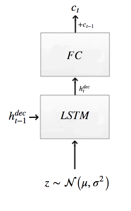
Sampling z and decode
# Sample from the distribution returned from the encoder to get z.
z = self.sample(self.mu[t], self.sigma[t], self.distrib)

# Get the hidden decoder state and the cell state using the a LSTM decoder.
h_dec, dec_state = self.decode_layer(dec_state, z)
The decoder composes of a LSTM cell.
def decode_layer(self, prev_state, latent):
    # update decoder RNN with latent var
    with tf.variable_scope("decoder", reuse=self.share_parameters):
       hidden_layer, next_state = self.lstm_dec(latent, prev_state)

    return hidden_layer, next_state
self.lstm_dec = tf.nn.rnn_cell.LSTMCell(self.n_hidden, state_is_tuple=True) # decoder Op
Output image
The output combines the previous output ct−1ct−1 with the output from FC layer.
# Calculate the output image at step t using attention with the decoder state as input.
self.ct[t] = c_prev + dense(hidden_layer, self.n_hidden, self.img_size**2)
To demonstrate how it is constructed, here is the code up to the encoder written in TensorFlow with the following steps:
- Read the MNist data.
- Set up the configuration for the LSTM cell.
- Construct a placeholder for the image.
- Construct the encoder and decoder operation.
- Construct the initial state (zero state) for the encoder and decoder.
- Unroll LSTM into T steps.
- Construct the encoder and decoder node at each time step.
class Draw():
    def __init__(self):
        # Read 55K of MNist training data + validation data + testing data
        self.mnist = input_data.read_data_sets("MNIST_data/", one_hot=True)
        self.n_samples = self.mnist.train.num_examples

        self.img_size = 28   # MNist is a 28x28 image
        self.N = 64          # Batch size used in the gradient descent.

        # LSTM configuration
        self.n_hidden = 256  # Dimension of the hidden state in each LSTM cell. (num_units in a TensorFlow LSTM cell)
        self.n_z = 10        # Dimension of the Latent vector
        self.T = 10          # Number of un-rolling time sequence in LSTM.

        # Attention configuration
        self.attention_n = 5 # Form a 5x5 grid for the attention.

        self.share_parameters = False  # Use in TensorFlow. Later we set to True so LSTM cell shares parameters.

        # Placeholder for images
        self.images = tf.placeholder(tf.float32, [None, 784])                  # image: 28 * 28 = 784

        # Create a random gaussian distrubtion we used to sample the latent variables (z).
        self.distrib = tf.random_normal((self.N, self.n_z), mean=0, stddev=1)  # (N, 10)

        # LSTM encoder and decoder
        self.lstm_enc = tf.nn.rnn_cell.LSTMCell(self.n_hidden, state_is_tuple=True)  # encoder Op
        self.lstm_dec = tf.nn.rnn_cell.LSTMCell(self.n_hidden, state_is_tuple=True)  # decoder Op
        self.ct = [0] * self.T        # Image output at each time step (T, ...) -> (T, N, 784)

        # Mean, log siggma and signma used for each unroll time step.
        self.mu, self.logsigma, self.sigma = [0] * self.T, [0] * self.T, [0] * self.T

        # Initial state (zero-state) for LSTM.
        h_dec_prev = tf.zeros((self.N, self.n_hidden))  # Prev decoder hidden state (N, 256)
        enc_state = self.lstm_enc.zero_state(self.N, tf.float32) # (64, 256)
        dec_state = self.lstm_dec.zero_state(self.N, tf.float32)

        x = self.images
        for t in range(self.T):

            # Calculate the input of LSTM cell with attention.
            # This is a function of
            #    the original image,
            #    the residual difference between previous output at the last time step and the original, and
            #    the hidden decoder state for the last time step.
            c_prev = tf.zeros((self.N, 784)) if t == 0 else self.ct[t - 1]  # (N, 784)
            x_hat = x - tf.sigmoid(c_prev)  # residual: (N, 784)
            r = tf.concat([x,x_hat], 1)

            # Using LSTM cell to encode the input with the encoder state
            # We use the attention input r and the previous decoder state as the input to the LSTM cell.
            self.mu[t], self.logsigma[t], self.sigma[t], enc_state = self.encode(enc_state, tf.concat([r, h_dec_prev], 1))

            # Sample from the distribution returned from the encoder to get z.
            z = self.sample(self.mu[t], self.sigma[t], self.distrib)

            # Get the hidden decoder state and the cell state using the a LSTM decoder.
            h_dec, dec_state = self.decode_layer(dec_state, z)

            # Calculate the output image at step t using attention with the decoder state as input.
            self.ct[t] = c_prev + self.write_attention(h_dec)

            # Update previous hidden state
            h_dec_prev = h_dec
            self.share_parameters = True  # from now on, share variables

        # Output the final output in the final timestep as the generated images
        self.generated_images = tf.nn.sigmoid(self.ct[-1])
Final image
Output the final image:
# Output the final output in the final timestep as the generated images
self.generated_images = tf.nn.sigmoid(self.ct[-1])
Attention implementation
The attention comes in 2 steps. In the first step, we use a fully connected (FC) network to predict the region of the attention from hdect−1ht−1dec and in the second step, we represent the attention region with grid points.
We replace the input of the encoder:
with a attention (the red rectangle):
In the code below, we call self.attn_window to predict the center of the attention area gx,gygx,gy using a FC network.
Draw use a FC network to compute a center point, sigma, distance for the grids.
def read_attention(self, x, x_hat, h_dec_prev):
    Fx, Fy, gamma = self.attn_window("read", h_dec_prev)     # (N, 5, 28),(N, 5, 28),(N,1)
    ...

# Given a hidden decoder layer: locate where to put attention filters
def attn_window(self, scope, h_dec):
    # Use a linear network to compute the center point, sigma, distance for the grids.
    with tf.variable_scope(scope, reuse=self.share_parameters):
        parameters = dense(h_dec, self.n_hidden, 5)    # (N, 5)

    # gx_, gy_: center of 2d gaussian on a scale of -1 to 1
    gx_, gy_, log_sigma2, log_delta, log_gamma = tf.split(parameters, 5, 1)     # (N, 1)
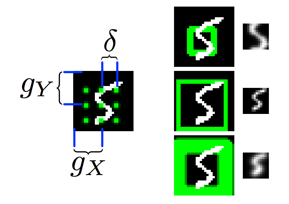
We can simply crop the attention area, rescale it to a standard size rectangle and then feed it into the encoder. But in DRAW, the attention area is instead represented by mxmmxm grid values (mxmmxm scalar values). In the example above, m=3m=3 and it generates a total of 9 grid points. Besides gx,gygx,gy, the FC also generate a δδ to indicate the distance between the grid points and a σσ for a gaussian filter. We apply the Gaussian filter over the image at each grid point to generate one single scalar value. Hence, the attention area will be represented by 9 grid points. In our code example, we will use m=5m=5 with 25 grid points. Here is the code in finding gx,gygx,gy, σσ and δδ from a FC network. Then we call filterbank to create gaussian filters that applied to the image later.
# Given a hidden decoder layer: locate where to put attention filters
def attn_window(self, scope, h_dec):
    # Use a linear network to compute the center point, sigma, distance for the grids.
    with tf.variable_scope(scope, reuse=self.share_parameters):
        parameters = dense(h_dec, self.n_hidden, 5)    # (N, 5)

    # gx_, gy_: center of 2d gaussian on a scale of -1 to 1
    gx_, gy_, log_sigma2, log_delta, log_gamma = tf.split(parameters, 5, 1)     # (N, 1)

    # move gx/gy to be a scale of -imgsize to +imgsize
    gx = (self.img_size + 1) / 2 * (gx_ + 1)   # (N, 1)
    gy = (self.img_size + 1) / 2 * (gy_ + 1)   # (N, 1)

    sigma2 = tf.exp(log_sigma2)  # (N, 1)

    # stride/delta: how far apart these patches will be
    delta = (self.img_size - 1) / ((self.attention_n - 1) * tf.exp(log_delta))   # (N, 1)

    # returns [Fx, Fy] Fx, Fy: (N, 5, 28)
    return self.filterbank(gx, gy, sigma2, delta) + (tf.exp(log_gamma),)
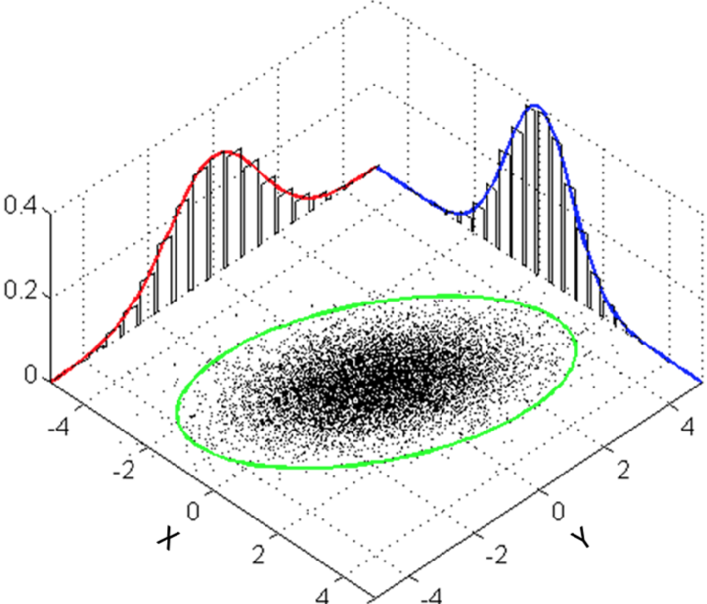
Our Gaussian distribution is symmetrical in 2-D. Therefore, we do not need filterbank to return a 2D filters. Instead, it returns 2 linear filters Fx,FyFx,Fy.
Source Wikipedia:
The shape of Fx,FyFx,Fy is (N, 5, 28) which N is the number of the batching datapoints. The output scalar value is computed by multiply (element wise) FxFx with a row of image data. Hence, the width of FxFx is 28.
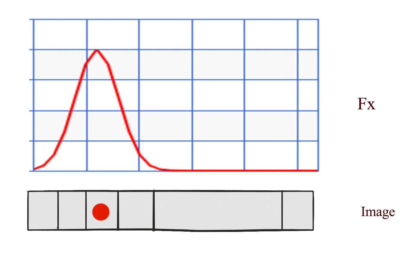
In additional, we have 5 grid points per row to generate 5 scalar values. Therefore, FxFx is (N, 5, 28).
# Given a center (gx, gy), sigma (sigma2) & distance between grid (delta)
# Construct gaussian filter grids (5x5) represented by Fx = horiz. gaussian (N, 5, 28), Fy = vert. guassian (N, 5, 28)
def filterbank(self, gx, gy, sigma2, delta):
    # Create 5 grid points around the center based on distance:
    grid_i = tf.reshape(tf.cast(tf.range(self.attention_n), tf.float32), [1, -1])  # (1, 5)
    mu_x = gx + (grid_i - self.attention_n / 2 - 0.5) * delta    # 5 grid points in x direction (N, 5)
    mu_y = gy + (grid_i - self.attention_n / 2 - 0.5) * delta

    mu_x = tf.reshape(mu_x, [-1, self.attention_n, 1])           # (N, 5, 1)
    mu_y = tf.reshape(mu_y, [-1, self.attention_n, 1])

   im = tf.reshape(tf.cast(tf.range(self.img_size), tf.float32), [1, 1, -1]) # (1, 1, 28)

   # list of gaussian curves for x and y
   sigma2 = tf.reshape(sigma2, [-1, 1, 1])               # (N, 1, 1)
   Fx = tf.exp(-tf.square((im - mu_x) / (2 * sigma2)))   # (N, 5, 28) Filter weight for each grid point and x_i
   Fy = tf.exp(-tf.square((im - mu_y) / (2 * sigma2)))

   # normalize so area-under-curve = 1
   Fx = Fx / tf.maximum(tf.reduce_sum(Fx, 2, keep_dims=True), 1e-8)    # (N, 5, 28)
   Fy = Fy / tf.maximum(tf.reduce_sum(Fy, 2, keep_dims=True), 1e-8)    # (N, 5, 28)
   return Fx, Fy
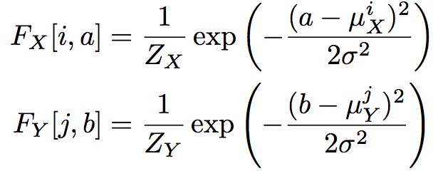
The position of the 5 grid points for x and y is:
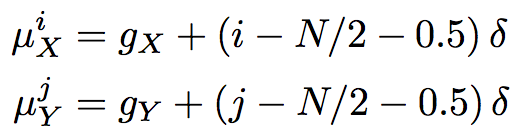
μixμxi is the ith grid point in the x-direction.
The Fx[i,a]Fx[i,a] (N, 5, 28) for the ithith grid point is computed as (aa is from pixel 0 to 27):
Here we replace:
with read_attention by applying Fx,FyFx,Fy over the image:
def read_attention(self, x, x_hat, h_dec_prev):
    Fx, Fy, gamma = self.attn_window("read", h_dec_prev)     # (N, 5, 28),(N, 5, 28),(N,1)

    # we have the parameters for a patch of gaussian filters. apply them.
    def filter_img(img, Fx, Fy, gamma):
        Fxt = tf.transpose(Fx, perm=[0, 2, 1])               # (N, 28, 5)
        img = tf.reshape(img, [-1, self.img_size, self.img_size]) # (N, 28, 28)
        glimpse = tf.matmul(Fy, tf.matmul(img, Fxt))                # (N, 5, 5)
        glimpse = tf.reshape(glimpse, [-1, self.attention_n ** 2])  # (N, 25)
        # finally scale this glimpse w/ the gamma parameter
        return glimpse * tf.reshape(gamma, [-1, 1])

    x = filter_img(x, Fx, Fy, gamma)                     # (N, 25)
    x_hat = filter_img(x_hat, Fx, Fy, gamma)             # (N, 25)
    return tf.concat([x, x_hat], 1)
Attention does not only apply to the input area but also to the output. We use another FC network to compute another attention area to indicate where we should write the output area to. We replace
def write_attention(self, hidden_layer):
    with tf.variable_scope("writeW", reuse=self.share_parameters):
        w = dense(hidden_layer, self.n_hidden, self.attention_n ** 2)
    w = tf.reshape(w, [self.N, self.attention_n, self.attention_n])
    Fx, Fy, gamma = self.attn_window("write", hidden_layer)
    Fyt = tf.transpose(Fy, perm=[0, 2, 1])
    # [vert, attn_n] * [attn_n, attn_n] * [attn_n, horiz]
    wr = tf.matmul(Fyt, tf.matmul(w, Fx))
    wr = tf.reshape(wr, [self.N, self.img_size ** 2])
    return wr * tf.reshape(1.0 / gamma, [-1, 1])
Cost function
To measure the lost between the orignal images and the generated images, (generation loss):
self.generation_loss = tf.reduce_mean(-tf.reduce_sum(
            self.images * tf.log(1e-10 +
			self.generated_images) +
			(1 - self.images) * tf.log(1e-10 + 1 - self.generated_images),
			1))
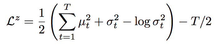
We use the KL divergence to measure the latent loss:
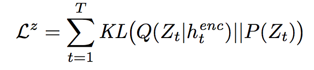
# Similar to the variation autoencoder, we add the KL divergence of the encoder distribution to the cost.
kl_terms = [0] * self.T                # list of 10 elements: each element (N,)
for t in range(self.T):
    mu2 = tf.square(self.mu[t])        # (N, 10)
    sigma2 = tf.square(self.sigma[t])  # (N, 10)
    logsigma = self.logsigma[t]        # (N, 10)
    kl_terms[t] = 0.5 * tf.reduce_sum(mu2 + sigma2 - 2 * logsigma, 1) - self.T * 0.5
self.latent_loss = tf.reduce_mean(tf.add_n(kl_terms)) # Find mean of (N,)
Result
The complet source coder can be found in the Github. Here is the image generated from GIF at different time step. With attention, we generate the image as if we are drawing with a pen.
Source Eric Jang
Credits
This article is based on Google Deepmind’s paper with explanation and source code started from the following blog:
Recommend
About Joyk
Aggregate valuable and interesting links.
Joyk means Joy of geeK