理解pytorch的计算逻辑

1 线性回归问题

假定我们以一个线性回归问题来逐步解释pytorch过程中的一些操作和逻辑。线性回归公式如下

y=a+bx+e此处假定a=1,b=2的一个线性回归函数y=a+bx+e此处假定a=1,b=2的一个线性回归函数

1.1 先用普通的numpy来展示线性回归过程

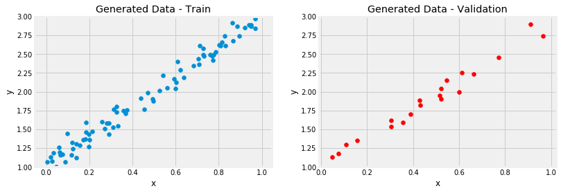
我们随机生成100个数据，并以一定的随机概率扰动数据集，训练集和验证集八二分，如下

# Data Generation
np.random.seed(42)
x = np.random.rand(100, 1)
y = 1 + 2 * x + .1 * np.random.randn(100, 1)

# Shuffles the indices
idx = np.arange(100)
np.random.shuffle(idx)

# Uses first 80 random indices for train
train_idx = idx[:80]
# Uses the remaining indices for validation
val_idx = idx[80:]

# Generates train and validation sets
x_train, y_train = x[train_idx], y[train_idx]
x_val, y_val = x[val_idx], y[val_idx]

上面这是我们已经知道的是一个线性回归数据分布，并且回归的参数是a=1,b=2a=1,b=2，如果我们只知道数据x_train和y_train，需要求这两个参数a,ba,b呢，一般是使用梯度下降方法。

注意，下面的梯度下降方法是全量梯度，一次计算了所有的数据的梯度，只是在迭代了1000个epoch，通常训练时会把全量数据分成多个batch，每次都是小批量更新。

# 初始化线性回归的参数 a 和 b
np.random.seed(42)
a = np.random.randn(1)
b = np.random.randn(1)
print("初始化的 a : %d 和 b : %d"%(a,b))
leraning_rate = 1e-2
epochs = 1000
for epoch in range(epochs):
    pred = a+ b*x_train
    # 计算预测值和真实值之间的误差
    error = y_train-pred
    # 使用MSE 来计算回归误差
    loss = (error**2).mean()
    # 计算参数 a 和 b的梯度
    a_grad = -2*error.mean()
    b_grad = -2*(x_train*error).mean()
    # 更新参数：用学习率和梯度
    a = a-leraning_rate*a_grad
    b = b -leraning_rate*b_grad

print("最终获得参数为 a : %.2f, b :%.2f "%(a,b))

得到的输出如下

初始化的 a : 0 和 b : 0
最终获得参数为 a : 0.98, b :1.94

再验证下是否与sklearn的LinearRegression回归算法得到的结果相同。

# 检查下，我们获得结果是否与sklearn的结果一致
from sklearn.linear_model import LinearRegression
linr = LinearRegression()
linr.fit(x_train,y_train)
print(linr.intercept_,linr.coef_[0])

得到的参数如下

[0.98312156] [1.94067463]

2 pytorhc 来解决回归问题

2.1 pytorch的一些基础问题

如果将numpy数组转化为pytorch的tensor呢？使用torch.from_numpy(data)
如果想将计算的数据放入GPU计算：data.to(device)(其中的device就是GPU或cpu)
数据类型转换示例： data.float()
如果确定数据位于CPU还是GPU:data.type()会得到类似于torch.cuda.FloatTensor的结果，表明在GPU中
从GPU中把数据转化成numpy：先取出到cpu中，再转化成numpy数组。data.cpu().numpy()

2.2 使用pytorch构建参数

如何区分普通数据和参数/权重呢？需要计算梯度的是参数，否则就是普通数据。参数需要用梯度来更新，我们需要选项requires_grad=True。使用了这个选项就是告诉pytorch，我们要计算此变量的梯度了。

我们可以使用如下三种方式来构建参数

此方法构建出来的参数全部都在cpu中

a = torch.randn(1, requires_grad=True, dtype=torch.float)
b = torch.randn(1, requires_grad=True, dtype=torch.float)
print(a, b)

此方法尝试把tensor参数传入到gpu

a = torch.randn(1, requires_grad=True, dtype=torch.float).to(device)
b = torch.randn(1, requires_grad=True, dtype=torch.float).to(device)
print(a, b)

此时如果查看输出，会发现两个tensor ，a和ba和b的梯度选项没了（没了requires_grad=True）

tensor([0.5158], device='cuda:0', grad_fn=<CopyBackwards>) tensor([0.0246], device='cuda:0', grad_fn=<CopyBackwards>)

先将tensor传入gpu，然后再使用requires_grad_()选项来重构tensor的属性。

a = torch.randn(1, dtype=torch.float).to(device)
b = torch.randn(1, dtype=torch.float).to(device)
# and THEN set them as requiring gradients...
a.requires_grad_()
b.requires_grad_()
print(a, b)

最佳策略当然是初始化的时候直接赋予requires_grad=True属性了

# We can specify the device at the moment of creation - RECOMMENDED!
torch.manual_seed(42)
a = torch.randn(1, requires_grad=True, dtype=torch.float, device=device)
b = torch.randn(1, requires_grad=True, dtype=torch.float, device=device)
print(a, b)

查看tensor的属性

tensor([0.6226], device='cuda:0', requires_grad=True) tensor([1.4505], device='cuda:0', requires_grad=True)

2.3 自动求导 Autograd

Autograd是Pytorch的自动求导包，有了它，我们就不必担忧偏导数和链式法则等一系列问题。Pytorch计算所有梯度的方法是backward()。计算梯度之前，我们需要先计算损失，那么需要调用对应(损失)变量的求导方法，如loss.backward()。

计算所有变量的梯度(假设损失变量是loss): loss.back()
获取某个变量的实际的梯度值(假设变量为att):att.grad
由于梯度是累加的，每次用梯度更新参数之后，需要清零(假设梯度变量是att):att.zero_(),下划线是一种运算符，相当于直接作用于原变量上，等同于att=0(不要手动赋值，因为此过程可能涉及到GPU、CPU之间数据传输，容易出错)

我们接下来尝试下手工更新参数和梯度

lr = 1e-1
n_epochs = 1000

torch.manual_seed(42)
a = torch.randn(1, requires_grad=True, dtype=torch.float, device=device)
b = torch.randn(1, requires_grad=True, dtype=torch.float, device=device)

for epoch in range(n_epochs):
    yhat = a + b * x_train_tensor
    error = y_train_tensor - yhat
    loss = (error ** 2).mean()

# 这个是numpy的计算梯度的方式
    # a_grad = -2 * error.mean()
    # b_grad = -2 * (x_tensor * error).mean()

# 告诉pytorch计算损失loss，计算所有变量的梯度
    loss.backward()
    # Let's check the computed gradients...
    print(a.grad)
    print(b.grad)  

# 1. 手动更新参数，会出错 AttributeError: 'NoneType' object has no attribute 'zero_'
    # 错误的原因是，我们重新赋值时会丢掉变量的 梯度属性
    # a = a - lr * a.grad
    # b = b - lr * b.grad
    # print(a)
    # 2. 再次手动更新参数，这次我们没有重新赋值，而是使用in-place的方式赋值  RuntimeError: a leaf Variable that requires grad has been used in an in- place operation.
    # 这是因为 pytorch 给所有需要计算梯度的python操作以及依赖都纳入了动态计算图，稍后会解释
    # a -= lr * a.grad
    # b -= lr * b.grad        

# 3. 如果我们真想手动更新，不使用pytorch的计算图呢，必须使用no_grad来将此参数移除自动计算梯度变量之外。
    # 这是源于pytorch的动态计算图DYNAMIC GRAPH，后面会有详细的解释
    with torch.no_grad():
        a -= lr * a.grad
        b -= lr * b.grad

# PyTorch is "clingy" to its computed gradients, we need to tell it to let it go...
    a.grad.zero_()
    b.grad.zero_()

print(a, b)

2.4 动态计算图

如果想可视化计算图，可以使用辅助包torchviz，需要自己安装。使用其make_dot(变量)方法来可视化与当前给定变量相关的计算图。示例

torch.manual_seed(42)
a = torch.randn(1, requires_grad=True, dtype=torch.float, device=device)
b = torch.randn(1, requires_grad=True, dtype=torch.float, device=device)

yhat = a + b * x_train_tensor
error = y_train_tensor - yhat
loss = (error ** 2).mean()
make_dot(yhat)

使用make_dot(yhat)会得到相关的三个计算图如下

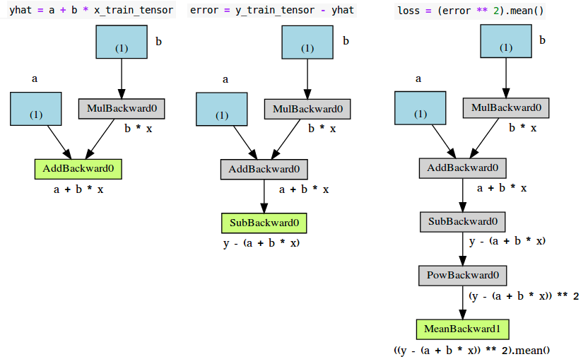
各个组件，解释如下

蓝色盒子：作为参数的tensor，需要pytorch计算梯度的
灰色盒子：与计算梯度相关的或者计算梯度依赖的，python操作
绿色盒子：与灰色盒子一样，区别是，它是计算梯度的起始点（假设backward()方法是需要可视化图的变量调用的）-计算图自底向上构建。

上图的error(图中)和loss(图右)，与左图的唯一区别就是中间步骤(灰色盒子)的数目。看左边的绿色盒子，有两个箭头指向该绿色盒子，代表两个变量相加。a和b*x。再看该图中的灰色盒子，它执行的是乘法计算，即b*x，但是为啥只有一个箭头指向呢，只有来自蓝色盒子的参数b，为啥没有数据x?因为我们不需要为数据x计算梯度（不计算梯度的变量不会出现在计算图中）。那么，如果我们去掉变量的requires_grad属性(设置为False)会怎样？

a_nongrad = torch.randn(1,requires_grad=False,dtype=torch.float,device=device)
b = torch.randn(1,requires_grad=True,dtype=torch.float,device=device)
yhat = a_nongrad+b*x_train_tensor

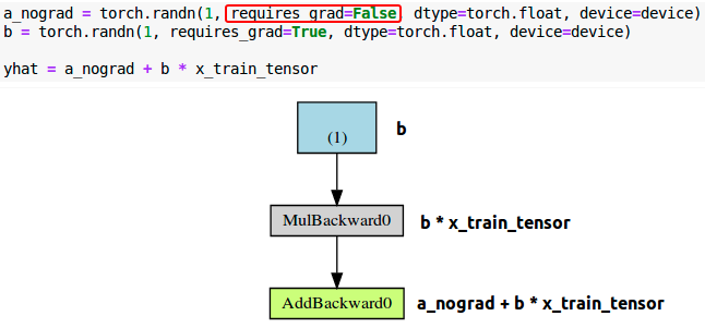
可以看到，对应参数a的蓝色盒子没有了，所以很简单明了，不计算梯度，就不出现在计算图中。

3 优化器 Optimizer

到目前为止，我们都是手动计算梯度并更新参数的，如果有非常多的变量。我们可以使用pytorch的优化器，像SGD或者Adam。

优化器需要指定需要优化的参数，以及学习率，然后使用step()方法来更新，此外，我们不必再一个个的去将梯度赋值为0了，只需要使用优化器的zero_grad()方法即可。。

代码示例，使用SGD优化器更新参数a和b的梯度。

torch.manual_seed(42)
a = torch.randn(1, requires_grad=True, dtype=torch.float, device=device)
b = torch.randn(1, requires_grad=True, dtype=torch.float, device=device)
print(a, b)

lr = 1e-1
n_epochs = 1000

# Defines a SGD optimizer to update the parameters
optimizer = optim.SGD([a, b], lr=lr)

for epoch in range(n_epochs):
    # 第一步，计算损失
    yhat = a + b * x_train_tensor
    error = y_train_tensor - yhat
    loss = (error ** 2).mean()
    # 第二步，后传损失
    loss.backward()    

# 不用再手动更新参数了
    # with torch.no_grad():
    # a -= lr * a.grad
    # b -= lr * b.grad
    # 使用优化器的step方法一步到位
    optimizer.step()

# 也不用告诉pytorch需要对哪些梯度清零操作了，优化器的zero_grad()一步到位
    # a.grad.zero_()
    # b.grad.zero_()
    optimizer.zero_grad()

print(a, b)

4 计算损失loss

pytorch提供了很多损失函数，可以直接调用。简单使用如下

torch.manual_seed(42)
a = torch.randn(1, requires_grad=True, dtype=torch.float, device=device)
b = torch.randn(1, requires_grad=True, dtype=torch.float, device=device)
print(a, b)

lr = 1e-1
n_epochs = 1000

# 此处定义了损失函数为MSE
loss_fn = nn.MSELoss(reduction='mean')

optimizer = optim.SGD([a, b], lr=lr)

for epoch in range(n_epochs):
    yhat = a + b * x_train_tensor

# 不用再手动计算损失了
    # error = y_tensor - yhat
    # loss = (error ** 2).mean()
    # 直接调用定义好的损失函数即可
    loss = loss_fn(y_train_tensor, yhat)

loss.backward()    
    optimizer.step()
    optimizer.zero_grad()

print(a, b)

pytorch中模型由一个继承自Module的Python类来定义。需要实现两个最基本的方法

__init__(self):定义了模型由哪几部分组成，当前模型只有两个变量a和b。模型可以定义更多的参数，并且可以将其他模型或者网络层定义为其参数
forwad(self,x):真实执行计算的方法，它对给定输入x输出模型预测值。不要显示调用此forward(x)方法，而是直接调用模型本身，即model(x)。

简单的回归模型如下

class ManualLinearRegression(nn.Module):
    def __init__(self):
        super().__init__()
        # To make "a" and "b" real parameters of the model, we need to wrap them with nn.Parameter
        self.a = nn.Parameter(torch.randn(1, requires_grad=True, dtype=torch.float))
        self.b = nn.Parameter(torch.randn(1, requires_grad=True, dtype=torch.float))

def forward(self, x):
        # Computes the outputs / predictions
        return self.a + self.b * x

在__init__(self)方法中，我们使用Parameters()类定义了两个参数a和b，告诉Pytorch，这两个tensor要被作为模型的参数的属性。这样，我们就可以使用模型的parameters()方法来找到模型每次迭代时的所有参数值了，即便模型是嵌套模型都可以找得到，这样就能将参数喂入优化器optimizer来计算了(而非手动维护一张参数表)。并且，我们可以使用模型的state_dict()方法来获取所有参数的当前值。

注意：模型应当与数据出于相同位置(GPU/CPU)，如果数据时GPU tensor，我们的模型也必须在GPU中

代码示例如下:

torch.manual_seed(42)

# Now we can create a model and send it at once to the device
model = ManualLinearRegression().to(device)
# We can also inspect its parameters using its state_dict
print(model.state_dict())

lr = 1e-1
n_epochs = 1000

loss_fn = nn.MSELoss(reduction='mean')
optimizer = optim.SGD(model.parameters(), lr=lr)

for epoch in range(n_epochs):
    #  注意，模型一般都有个train()方法，但是不要手动调用，此处只是为了说明此时是在训练，防止有些模型在训练模型和验证模型时操作不一致，训练时有dropout之类的
    model.train()

# No more manual prediction!
    # yhat = a + b * x_tensor
    yhat = model(x_train_tensor)

loss = loss_fn(y_train_tensor, yhat)
    loss.backward()    
    optimizer.step()
    optimizer.zero_grad()

print(model.state_dict())

我们定义了optimizer,loss function,model为模型三要素，同时需要提供训练时用的特征(feature)和对应的标签(label)数据。一个完整的模型训练有以下组成

模型三要素
- 优化器optimizer
- 损失函数loss
- 模型 model
数据
- 特征数据feature
- 数据标签label

我们可以写一个包含模型三要素的通用的训练函数

def make_train_step(model, loss_fn, optimizer):
    # Builds function that performs a step in the train loop
    def train_step(x, y):
        # Sets model to TRAIN mode
        model.train()
        # Makes predictions
        yhat = model(x)
        # Computes loss
        loss = loss_fn(y, yhat)
        # Computes gradients
        loss.backward()
        # Updates parameters and zeroes gradients
        optimizer.step()
        optimizer.zero_grad()
        # Returns the loss
        return loss.item()

# Returns the function that will be called inside the train loop
    return train_step

然后在每个epoch时迭代模型训练

# Creates the train_step function for our model, loss function and optimizer
train_step = make_train_step(model, loss_fn, optimizer)
losses = []

# For each epoch...
for epoch in range(n_epochs):
    # Performs one train step and returns the corresponding loss
    loss = train_step(x_train_tensor, y_train_tensor)
    losses.append(loss)

# Checks model's parameters
print(model.state_dict())

medium understand pytorch

1 线性回归问题

1.1 先用普通的numpy来展示线性回归过程

2 pytorhc 来解决回归问题

2.1 pytorch的一些基础问题

2.2 使用pytorch构建参数

2.3 自动求导 Autograd

2.4 动态计算图

3 优化器 Optimizer

4 计算损失loss

Recommend

近端算子求解分布式约束优化问题

Issue #1: Project Updates, DBUI, and Interesting Open Source Repositories

产品经理如何做即兴演讲

互联网之子:亚伦·斯沃茨的故事

JCommander：Java外部参数解析利器

Potato dauphinoise

Kanan Rahimov (KenanBek)

萨摩耶云杜亚威：云原生+AI打造决策最优路径

Accessible forms with ARIA live regions

Domain-Driven Design to the rescue

About Joyk