Mathematics is the foundation on which machine learning is build. We will refresh few basic concepts to get started.

Vectors

Vector is a construct that represents both a direction as well as a magnitude. Algebraically, a vector is the collection of coordinates that a point has in a given space. Geometrically, vector is a ray that connects origin to the point.

Following figure shows examples of vectors in two dimensional Euclidean space.

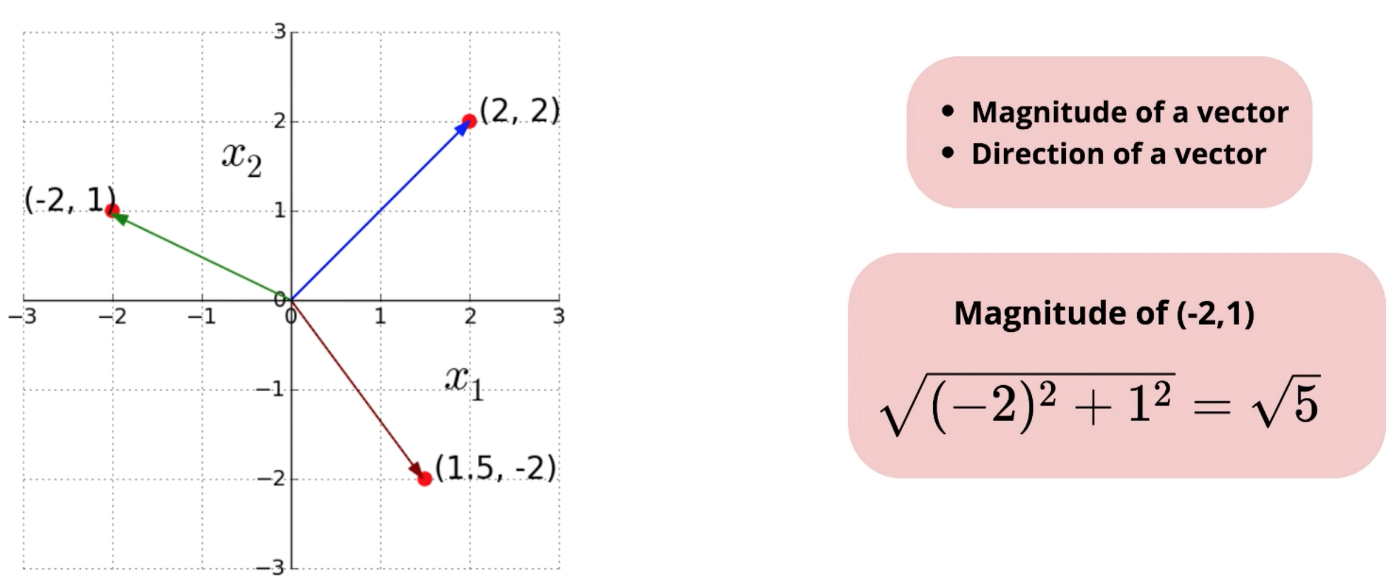
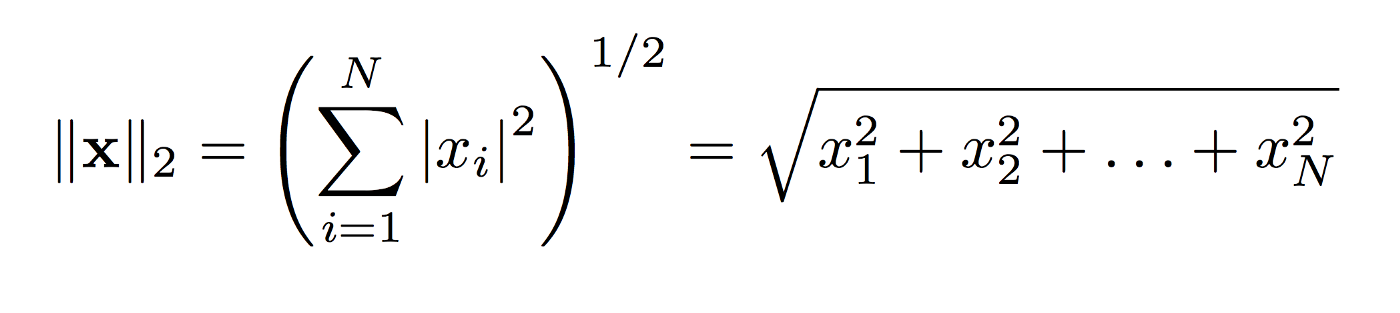
L2 norm calculates the distance of the vector coordinate from the origin of the vector space. It is also known as the Euclidean norm as it is calculated as the Euclidean distance from the origin. The result is a positive distance value.

The L2 norm is calculated as the square root of the sum of the squared vector values.

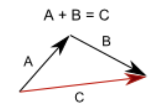
Addition and Subtraction

Vector addition is used to accumulate the difference described by both vectors into the final vector. For example, if an object moves by A vector, and then by B vector, the result is the same as if it would have moved by C vector.

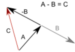
For Vector subtraction, the second vector is simply inverted and added to the first one.

Dot product

A dot product is an operation on two vectors, which returns a number, written as, A dot B.

Dot product represents a difference in rotation between vectors.

• If dot product is 1, vectors face the same direction.
• If dot product is 0, vectors are perpendicular.
• If dot product is -1, vectors face opposite directions.

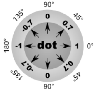
Change from 1 to 0 and from 0 to -1 is not linear, but follows a cosine curve. To get an angle from a dot product, you need to calculate arc-cosine of it: angle = acos(A dot B)

Cross Product

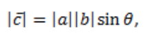
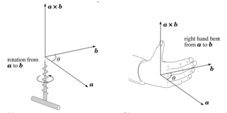
A cross product or vector product is an operation on two vectors. The result is a third vector, which is perpendicular to the first two vectors.

The magnitude of the cross product is given as:

The direction of the cross product is given as:

Unit Vector

A unit vector or normalized vector has magnitude 1. Simplest unit vector are in the direction of coordinate axis. In two dimension space, simplest unit vectors are (0, 1) and (1, 0).

A unit vector in the direction of a given vector can be found by dividing the vector by its norm.

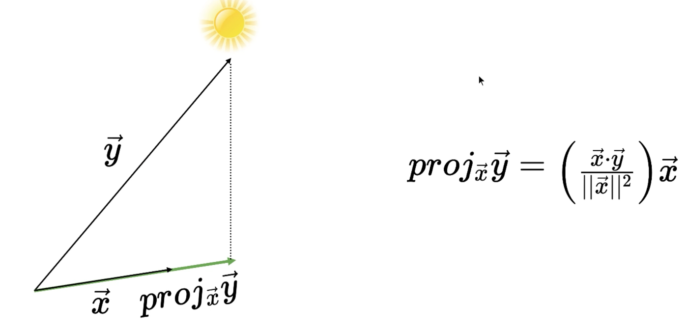
Projection

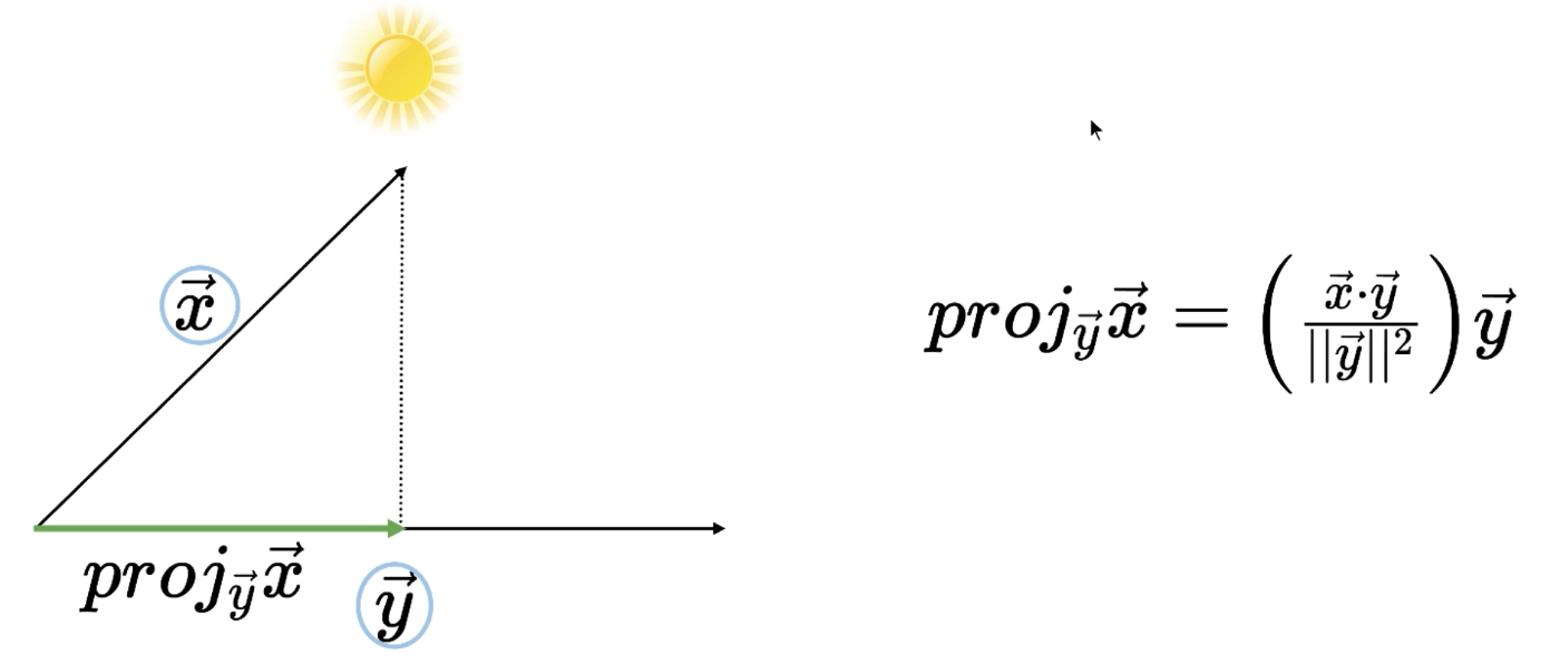
Projection can be considered as light shining from the top and one need to find how the shadow of one vector is seen on second vector.

It is given by formula shown below, which can be thought of as taking a unit vector in the direction of second vector and multiplying that with the dot product of two vectors.

Angle between two vectors

Matrices

Matrices is a collection of many vectors, known as row vectors and column vectors. Various operations are performed on Matrices namely addition, subtraction and multiplication.

Matrix multiplication with a vector

To multiply a matrix with a vector, number of columns in the matrix should be same as number of rows in the vector.

When a matrix is multiplied with a vector, the vector gets transformed into a new vector i.e. the new vector path is generally different and it can scaled up or down based on matrix values.

You can think of it as each row vector gets multiplied with the vector.

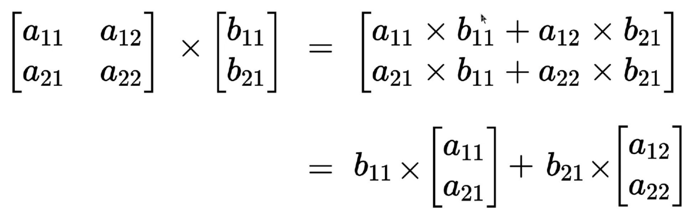
Matrix multiplication with a matrix

Any m x n matrix can be multiplied with a n x k matrix to get a m x k output i.e. number of columns of first matrix should be same as number of rows of second matrix.

When a matrix is multiplied with a matrix, it can be considered as a series of matrix-vector multiplication. It is the product of the first matrix with every column of the second matrix.

Alternate way to look at matrix multiplication is that the output is a linear combination of the columns of the first matrix and the weights are the elements of vector (or second matrix).

Probability Theory

Axioms

For any event A, 0 ≤ P(A) ≤ 1

• If A₁, A₂, A₃, … are disjoint events, then P(∪Aᵢ) = ∑ᵢ P(Aᵢ)
• If Ω is the universal set containing all events, then P(Ω) = 1

Random Variable

A random variable is a function which maps each outcome in universal set (Ω) to a value. As shown below, G, H and A are random variables mapping Ω to the set of Grades, Height and Age respectively.

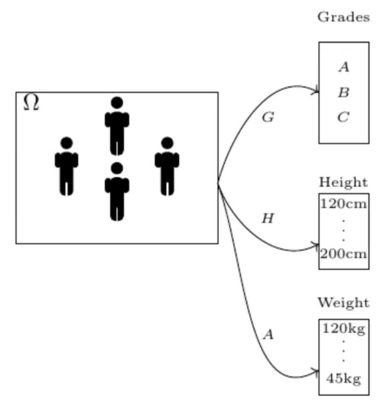
A random variable can either take continuous values (e.g. weight, height) or discrete values (e.g. grade). Accordingly, random variable is called continuous random variable or discrete random variable.

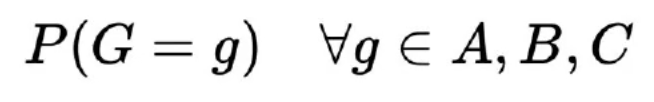
Marginal probability distribution

Marginal distribution or probability distribution over a discrete random variable is the table of probability for every value that random variable can take.

For example, in case students can get grades G having values A, B or C, the marginal distribution over G means

Information Theory

Information theory is a subfield of mathematics concerned with transmitting data across a noisy channel. Main idea of is to quantify how much information a message carries. This can be used to quantify the information in an event and a random variable, called entropy, and is calculated using probability.

Calculating information and entropy is useful in machine learning techniques like feature selection, decision trees, and optimization of classification models.

Expectation

The expected value of a random variable is defined as the weighted average of the values in the range.

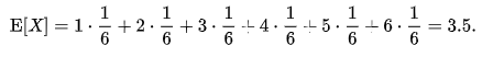
Let X represent the outcome of a roll of a fair six-sided die. The possible values for X are 1, 2, 3, 4, 5, and 6, all of which are equally likely with a probability of 1/6. The expectation of X is

Information Content

The basic idea of information theory is that the “informational value” of a communicated message depends on the degree to which the content of the message is surprising. If an event is very probable, it is no surprise when that event happens as expected; hence transmission of such a message carries very little new information. However, if an event is unlikely to occur, it is much more informative to learn that the event happened or will happen.

• Low Probability Event: High Information (surprising).
• High Probability Event: Low Information (unsurprising).

The amount of information for an event can be calculated using the probability of the event. This is called “Shannon information,” and can be calculated for a discrete event x as follows:

h(x) = -log( p(x) )

Where log() is the base-2 logarithm and p(x) is the probability of the event x.

Entropy of a Random Variable

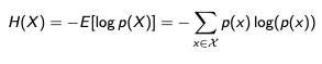
Entropy is the expected information content of a random variable.

Entropy can be calculated for a random variable X as follows:

The intuition for entropy is that

• It is the average number of bits required to represent or transmit an event drawn from the probability distribution for the random variable.
• It is the measure of average uncertainty in random variable.

Cross-Entropy

Cross-entropy is a measure of the difference between two probability distributions for a given random variable.

Cross-entropy builds upon the idea of entropy from information theory and calculates the number of bits required to represent or transmit an average event from one distribution compared to another distribution.

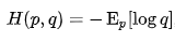
The cross-entropy of the distribution q relative to a distribution p over a given set is defined as follows:

The intuition for cross entropy is that

• Suppose P is the given or target probability distribution and Q is an approximation of the target distribution, then the cross-entropy of Q from P is the number of additional bits to represent an event using Q instead of P.

References: