Le Petit Chercheur Illustré

There is time for dithering in a quantized world of reduced dimensionality!

I’m glad to announce here a new work made in collaboration with Valerio Cambareri (UCL, Belgium) on quantized embeddings of low-complexity vectors, such as the set of sparse (or compressible) signals in a certain basis/dictionary, the set of low-rank matrices or vectors living in (a union of) subspaces.

The title and the abstract are as follows (arxiv link here).

“Time for dithering: fast and quantized random embeddings
via the restricted isometry property”

Recently, many works have focused on the characterization of non-linear dimensionality reduction methods obtained by quantizing linear embeddings, e.g., to reach fast processing time, efficient data compression procedures, novel geometry-preserving embeddings or to estimate the information/bits stored in this reduced data representation. In this work, we prove that many linear maps known to respect the restricted isometry property (RIP), can induce a quantized random embedding with controllable multiplicative and additive distortions with respect to the pairwise distances of the data points beings considered. In other words, linear matrices having fast matrix-vector multiplication algorithms (e.g., based on partial Fourier ensembles or on the adjacency matrix of unbalanced expanders), can be readily used in the definition of fast quantized embeddings with small distortions. This implication is made possible by applying right after the linear map an additive and random “dither” that stabilizes the impact of a uniform scalar quantization applied afterwards.
For different categories of RIP matrices, i.e., for different linear embeddings of a metric space $(\mathcal K \subset \mathbb R^n, \ell_q)$ in $(\mathbb R^m, \ell_p)$ with $p,q \geq 1$ , we derive upper bounds on the additive distortion induced by quantization, showing that this one decays either when the embedding dimension $m$ increases or when the distance of a pair of embedded vectors in $\mathcal K$ decreases. Finally, we develop a novel “bi-dithered” quantization scheme, which allows for a reduced distortion that decreases when the embedding dimension grows, independently of the considered pair of vectors.

In a nutshell, the idea of this article stems from the following observations. There is an ever-growing literature dealing with the design of quantized/non-linear random maps or data hashing techniques for reaching novel dimensionality reduction techniques. More particularly, inside it, some of the works are interested in the accurate control of the number of bits needed to encode the image of the maps, for instance by combining a random linear map with a quantization process approximating the continuous image of the linear map to a finite set of vectors (e.g., using a uniform or a 1-bit quantizer [1,2,3,4]). This quantization is indeed important for instance to reduce and bound the processing time of the quantized signal signatures obtained with this map. In fact, if the quantized map is also an embedding, i.e., if it preserves the pairwise distances of the mapped vectors up to some distortions, we can process the (compact) vector signatures as a proxy to the full processing we would like to perform on the original signals, e.g., for nearest neighbors search or machine learning algorithms.

However, AFAIK, either these random constructions embrace the embedding of general low-complexity vectors sets (possibly continuous) thanks to the quantization of (slow and unstructured) linear random projections (e.g., using a non-linear alteration/quantization of a linear projection reached by a sub-Gaussian random matrix with $O(mn)$ encoding complexity [1,2,3,4]), or they rely on fast non-linear maps (e.g., exploiting circulant random matrices) which are unfortunately restricted (up to now) to the embedding of finite vector sets [5,6,7].

This is rather frustrating when we know that the compressive sensing (CS) literature now offers us a large class of linear embeddings of low-complexity vector sets, i.e., including constructions with fast (possibly with log-linear complexity) projections of vectors. We can think for instance to the projections induced by partial Fourier/Hadamard ensembles [9], random convolutions [10] or the spread-spectrum sensing [11].

Adopting a general formulation federating several definitions available in different works, this embedding capability is mathematically characterized by the celebrated restricted isometry property (or RIP), i.e., a matrix $\boldsymbol \Phi \in \mathbb R^{m \times n}$ respects the $(\ell_p, \ell_2)$ -RIP $(\mathcal K - \mathcal K, \epsilon)$ with (multiplicative) distortion $\epsilon > 0$ , if for all $\boldsymbol x, \boldsymbol x' \in \mathcal K$ and some $p \in \{1,2\}$ ,

$(1-\epsilon) \|\boldsymbol x - \boldsymbol x'\|^p \leq \tfrac{1}{m} \|\boldsymbol \Phi(\boldsymbol x - \boldsymbol x')\|_p^p \leq (1+\epsilon) \|\boldsymbol x - \boldsymbol x'\|^p.$

Given such a matrix $\boldsymbol \Phi$ and a uniform quantization $\mathcal Q(\lambda) = \delta (\lfloor \tfrac{\lambda}{\delta}\rfloor + \tfrac{1}{2})$ (with resolution $\delta > 0$ ) applied componentwise onto vectors, we can define the quantized map $A'(\boldsymbol x) := \mathcal Q(\boldsymbol\Phi\boldsymbol x) \in \delta (\mathbb Z + \tfrac{1}{2})^m$ and easily observe (since $|\mathcal Q(\lambda) - \lambda| \leq \delta/2$ ) that

$(1-\epsilon)^{1/p} \|\boldsymbol x - \boldsymbol x'\| - \delta \leq \tfrac{1}{\sqrt[p] m} \|A'(\boldsymbol x) - A'(\boldsymbol x')\|_p \leq (1+\epsilon)^{1/p} \|\boldsymbol x - \boldsymbol x'\| + \delta.$

Strikingly, we observe now that, compared to the RIP that only displays a multiplicative distortion $\epsilon$ , this last relation contains now an additive — and constant! — distortion $\delta$ , which is the direct expression of the quantization process.

However, our work actually shows that it is nevertheless possible to design quantized embeddings where this new additive distortion can be controlled (and reduced) with either the dimension $m$ of the embedding domain or with the distance $\|\boldsymbol x - \boldsymbol x'\|$ of the considered points.

The key is to combine a linear embeddings $\boldsymbol \Phi$ (i.e., satisfying the $(\ell_p, \ell_2)$ -RIP) with a dithered and uniform quantization process [8], i.e., we insert $m$ iid uniform random variables on each component of the linear map before quantization. Notice that once randomly generated, as for $\boldsymbol \Phi$ , these dithers must of course be stored. However, such a storage is small (or at most comparable) to the the storage of a RIP matrix, i.e., we must anyway record $O(mn)$ entries for unstructured matrices and $O(m)$ values for the lightest structured constructions [9,11,15]. Noticeably, several works already included this dithering procedure as a way to ease the statistical analysis of the resulting map (see, e.g., the constructions defined for universal embeddings [12], the random Fourier features [13] or for locality preserving hashing [4,14]).

Roughly speaking (see the paper for the correct statements), among other things, we show that if a matrix $\boldsymbol \Phi \in \mathbb R^{m \times n}$ respects the $(\ell_p, \ell_2)$ -RIP $(\mathcal K - \mathcal K, \epsilon)$ , then, provided $m$ is larger than the $\epsilon'$ -Kolmogorov entropy of $\mathcal K$ with $\epsilon' = \epsilon'(\epsilon)$ being some power of $\epsilon$ (i.e., for the set of $k$ -sparse vectors in $\mathbb R^n$ , this would mean that $m= O\big({\epsilon}^{-2} k \log(n/\delta\epsilon^2 k)\big)$ ), the map $A: \mathbb R^n \to \mathcal E := \delta (\mathbb Z + 1/2)^m$ defined by

$A(\boldsymbol x) := \mathcal Q(\boldsymbol \Phi \boldsymbol x + \boldsymbol \xi), \quad \mathcal Q(\lambda) = \delta (\lfloor \tfrac{\lambda}{\delta}\rfloor + \tfrac{1}{2}),\ \xi_i \sim_{\rm iid} \mathcal U([0,\delta])$

is such that, with high probability and given a suitable concept of (pre)metric $d_{\mathcal E}$ in $\mathcal E$ ,

$d_{\mathcal E}(A(\boldsymbol x), A(\boldsymbol x')) \approx \|\boldsymbol x - \boldsymbol x'\|^p,\quad \forall \boldsymbol x, \boldsymbol x' \in \mathcal K,$

where the approximation symbol hides an additive and a multiplicative errors (or distortions).

More precisely, we have with high probability a quantized form of the RIP, or $(d_{\mathcal E}, \ell_2)$ -QRIP $(\mathcal K, \epsilon, \rho)$ , that reads

$(1-\epsilon) \|\boldsymbol x - \boldsymbol x'\|^p - \rho \leq d_{\mathcal E}(A(\boldsymbol x), A(\boldsymbol x')) \leq (1+\epsilon) \|\boldsymbol x - \boldsymbol x'\|^p + \rho,$

for all $\boldsymbol x, \boldsymbol x' \in \mathcal K$ and some distortions $\epsilon$ and $\rho = \rho(\epsilon, \|\boldsymbol x - \boldsymbol x'\|)$ .

Interestingly enough, this last additive distortion $\rho$ — a pure effect of the quantization in the definition of $A$ since the linear RIP is not subject to it — truly depends on the way distances are measured both in $\mathbb R^m$ (for the range of $\boldsymbol \Phi$ ) and in $\mathcal E$ .

For instance, if one decides to measure the distances with the $\ell_1$ -norm ( $p = 1$ ) in these both domains, hence asking $\boldsymbol \Phi$ to respect a $(\ell_1, \ell_2)$ -RIP, we have

$\rho\ \lesssim\ \delta \epsilon,$

as explained in Prop. 1 of our work.

If we rather focus on using $(\ell_2, \ell_2)$ -RIP matrices for defining the quantized map $A$ (hence allowing for fast and structured constructions) and on measuring the distances with squared $\ell_2$ -norm in both $\mathbb R^m$ and $\mathcal E$ , then

$\rho(\epsilon, s)\ \lesssim\ \delta s + \delta^2 \epsilon,$

where $s$ stands for the dependence in the distance. This is expressed in the Prop. 2 of our paper and it shows that for this particular choice of distances, the additive distortion is controllable and small compared to large values of $s^2 = \|\boldsymbol x - \boldsymbol x'\|^2$ , but it only tends to zero if both this distance and the resolution $\delta$ do so.

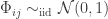
Bi-dithered quantized map: Desiring to preserve the inheritance of the $(\ell_2, \ell_2)$ -RIP matrix constructions in the construction of an efficient quantized embedding, i.e., with a smaller distortion $\rho$ than in the last scheme above, our paper also introduce a novel bi-dithered quantized map.

The principle is really simple. For each row of a RIP matrix, two dithers and thus two measurements are generated (hence doubling the total number $m$ of measurements). Mathematically, we now define the map $A: \mathbb R^n \to \mathcal E := \delta (\mathbb Z + \tfrac{1}{2})^{m \times 2}$ with

$\bar A(\boldsymbol x) := \mathcal Q(\boldsymbol \Phi \boldsymbol x \boldsymbol 1_2^T + \boldsymbol \Xi),\ \boldsymbol \Xi \in \mathbb R^{m \times 2},\ \Xi_{ij} \sim_{\rm iid} \mathcal U([0,\delta]),$

writing $\boldsymbol 1_2^T = (1\ 1)$ . Then, one can show, and this is Prop. 3 in our paper, that if $\mathbb R^m$ is endowed with the $\ell_2$ norm and $\mathcal E$ with the premetric $\|\cdot\|_{1,\circ}$ such that

$\| \boldsymbol B \|_{1,\circ} := \sum_i \Pi_j |B_{ij}|,\quad \boldsymbol B \in \mathbb R^{m \times 2},$

then, provided $m$ is again larger than the $\epsilon'$ -Kolmogorov entropy of $\mathcal K$ , the map $\bar A$ does also determine with high probability a quantized embedding of $\mathcal K$ in $\mathcal E$ with reduced additive distortion bounded as

$\rho(\epsilon, s)\ \lesssim\ \delta^2 \epsilon,$

which is much smaller than what is reached in the case of a single dither.

All these results are actually summarized in the following table extracted from the paper (the caption is better understood by reading the paper):

table

Remark 1 (connection with the “fast JL maps from RIP”-approach): The gist of our work is after all quite similar, in another context, to the standpoint adopted in this paper by Krahmer and Ward for the development of fast Johnson-Lindenstrauss embeddings using the large class of RIP matrix constructions (when combined with a random pre-modulating $\pm 1$ diagonal matrix) [17].

Remark 2 (on the proofs): The proofs developed in our work are not really technical and are all based on the same structure: the (variant of the) RIP allows us to focus on the embedding of the image of a low-complexity vector set (obtained through the corresponding linear map $\boldsymbol \Phi$ ) into a quantized domain thanks to a randomly dithered-quantization. This is made possible by softening the discontinuous distances evaluated in the quantized domain according to a mathematic machinery inspired by [3] in the case of 1-bit quantization and extended in [16] for dithered uniform scalar quantization (as above). Actually, this softening allows us to extend the concentration of quantized random maps on a finite covering of the low-complexity vector set $\mathcal K$ to this whole set by a continuity argument.

Remark 3 (on RIP-1 matrices): We do not mention in this post another variant of the RIP above, i.e., embedding $(\mathbb R^n, \ell_1)$ in $(\mathbb R^m, \ell_1)$ , that allows us also to inherit of the “RIP-1” matrices developed in [15] (associated to the adjacency matrix of expanders graphs) with distortion $\rho \lesssim \delta /epsilon$ .

Remark 4 (on 1-bit quantized embeddings): If the set $\mathcal K$ is bounded (e.g., as for the set of bounded sparse vectors), a careful selection of the quantization resolution $\delta > 0$ actually turns the map $A$ into a 1-bit embedding! Indeed, each of its components can basically take only two values if $\delta$ reaches the diameter of $\mathcal K$ .

Open problems:

Even if Remark 4 above shows us that 1-bit quantized embeddings are reachable with a dithered quantization of RIP-based linear embeddings, it is still an open and challenging problem to understand if fast embeddings can be designed with (undithered) sign operator [5,6,7].
A generalization of the bi-dithered quantized map above to a multi-dithered version (with of course a careful study of the corresponding increase of the measurement number) could potentially lead us to more advanced and distorted mappings, e.g., where distances are distorted by a polynomial of degree set by the number of dithers attributed to each row of $\boldsymbol \Phi$ .

References:

[1] P. T. Boufounos and R. G. Baraniuk. 1-bit compressive sensing. In Information Sciences and Systems, 2008. CISS 2008. 42nd Annual Conference on, pages 16–21. IEEE, 2008.
[2] L. Jacques, J. N. Laska, P. T. Boufounos, and R. G. Baraniuk. Robust 1-bit compressive sensing via binary stable embeddings of sparse vectors. Information Theory, IEEE Transactions on, 59(4):2082–2102, 2013.
[3] Y. Plan and R. Vershynin. Dimension reduction by random hyperplane tessellations. Dis- crete & Computational Geometry, 51(2):438–461, 2014.
[4] M. Datar, N. Immorlica, P. Indyk, and V. S. Mirrokni. Locality-sensitive hashing scheme based on p-stable distributions. In Proceedings of the twentieth annual symposium on Computational geometry, pages 253–262. ACM, 2004.
[5] S. Oymak. Near-Optimal Sample Complexity Bounds for Circulant Binary Embedding. arXiv preprint arXiv:1603.03178, 2016.
[6] F. X. Yu, A. Bhaskara, S. Kumar, Y. Gong, and S.-F. Chang. On Binary Embedding using Circulant Matrices. arXiv preprint arXiv:1511.06480, 2015.
[7] F. X. Yu, S. Kumar, Y. Gong, and S.-F. Chang. Circulant binary embedding. arXiv preprint arXiv:1405.3162, 2014.
[8] R. M. Gray and D. L. Neuhoff. Quantization. Information Theory, IEEE Transactions on, 44(6):2325–2383, 1998.
[9] H. Rauhut, J. Romberg, and J. A. Tropp. Restricted isometries for partial random circulant matrices. Applied and Computational Harmonic Analysis, 32(2):242–254, 2012.
[10] J. Romberg. Compressive sensing by random convolution. SIAM Journal on Imaging Sciences, 2(4):1098–1128, 2009.
[11] G. Puy, P. Vandergheynst, R. Gribonval, and Y. Wiaux. Universal and efficient compressed sensing by spread spectrum and application to realistic Fourier imaging techniques. EURASIP Journal on Advances in Signal Processing, 2012(1):1–13, 2012.
[12] P. T. Boufounos, S. Rane, and H. Mansour. Representation and Coding of Signal Geometry. arXiv preprint arXiv:1512.07636, 2015.
[13] A. Rahimi and B. Recht. Random features for large-scale kernel machines. In Advances in neural information processing systems, pages 1177–1184, 2007.
[14] A. Andoni and P.Indyk. Near-optimal hashing algorithms for approximate nearest neighbor in high dimensions. In Foundations of Computer Science, 2006. FOCS’06. 47th Annual IEEE Symposium on, pages 459–468. IEEE, 2006.
[15] R. Berinde, A. C. Gilbert, P. Indyk, H. Karloff, and M. J. Strauss. Combining geometry and combinatorics: A unified approach to sparse signal recovery. In Communication, Control, and Computing, 2008 46th Annual Allerton Conference on, pages 798–805. IEEE, 2008.
[16] L. Jacques. Small width, low distortions: quasi-isometric embeddings with quantized sub- Gaussian random projections. arXiv preprint arXiv:1504.06170, 2015.
[17] F. Krahmer, R. Ward, “New and improved Johnson-Lindenstrauss embeddings via the restricted isometry property”. SIAM Journal on Mathematical Analysis, 43(3), 1269-1281, 2011.

Quantized sub-Gaussian random matrices are still RIP!

I have always been intrigued by the fact that, in Compressed Sensing (CS), beyond Gaussian random matrices, a couple of other unstructured random matrices respecting, with high probability (whp), the Restricted Isometry Property (RIP) look like “quantized” version of the Gaussian case, i.e., their discrete entries have a probability density function (pdf) that seems induced by a discretized version of the Gaussian pdf.

For instance, two random constructions that are known to allow CS of sparse signals by respecting the RIP, namely the Bernoulli random matrix, with entries identically and independently distributed (iid) as a rv taking $\pm 1$ with equal probability, and the ternary matrix with iid random entries selected within $\{0, \pm 1\}$ with probability $2/3$ and $1/6$ [3], respectively, look like a certain “quantization” of a Gaussian pdf.

This short post aims simply to show that this fact can be easily understood thanks to known results showing that sub-Gaussian random matrices respect the RIP [3]. Certain of the relations described below are probably very well known in the statistical literature but, as we are always re-inventing the wheel (at least me ;-)), I found anyway interesting to share this through this blog post.

Let’s first recall what a sub-Gaussian random variable (rv) is. For this, I’m following [1]. A random variable $X$ is sub-Gaussian if its sub-Gaussian norm

$\|X\|_{\psi_2} := \sup_{p\geq 1} p^{-1/2}\,(\mathbb E |X|^p)^{1/p}$

is finite. In particular, any rv with such a finite norm has a tail bound that decays as fast as the one of a Gaussian rv, i.e., for some $c>0$ independent of $X$ , if $\|X\|_{\psi_2} \leq L$ , then

$\mathbb P[|X| \geq t] \lesssim \exp(- c t^2/L^2).$

The set of sub-Gaussian random variables includes for instance the Gaussian, the Bernoulli and the bounded rv’s, as $\|X\|_{\psi_2} \leq {\rm inf}\{t > 0: \mathbb P(|X|<t) = 1\}$ .

In CS theory, it is now well known that if a random matrix $\Phi \in \mathbb R^{M \times N}$ is generated randomly with iid entries drawn as a sub-Gaussian rv with zero mean and unit variance, then, with high probability and provided $M \gtrsim K \log N/K$ ,the matrix $\Phi$ respects the RIP of order $K$ and constant $\delta \in (0,1)$ , i.e.,

$\forall u \in \mathbb R^N: \|u\|_0 := |{\rm supp}\,u| \leq K,\ (1-\delta)\|u\| \leq \|\Phi u\| \leq (1+\delta) \|u\|.$

In fact, if $\Phi$ has the RIP $(2K,\delta)$ , any $K$ -sparse signal $x$ (with $\|x\|_0 \leq K$ ) can be stably estimated (e.g., using Basis Pursuit or greedy algorithms) from $y = \Phi x + n$ , possibly with some moderate noise $n$ [2].

The simple point I’d like to show here is that a large class of RIP matrices can be generated by quantizing (elementwise) Gaussian and sub-Gaussian random matrices. I’m going to show this by proving that (i) quantizing a Gaussian rv leads to a sub-Gaussian rv, (ii) its sub-Gaussian norm can be easily upper bounded.

But what do I mean by “quantizing”?

This operation is actually defined here through a partition $\mathcal P = \{\mathcal P_i: i \in \mathbb Z\}$ of $\mathbb R$ , i.e., $\mathcal P_i \cap \mathcal P_j = \emptyset$ if $i \neq j$ and $\cup_i \mathcal P_i = \mathbb R$ .

Given a rv $X$ , this partition determines a set of countable levels (or codebook) $\mathcal C =\{c_i: i\in \mathbb Z\}$ such that

$c_i(X) := \mathbb E[X|\mathcal P_i] = \mathbb E[X|X\in \mathcal P_i].$

The quantized version $Z = \mathcal Q(X)$ of $X$ is then defined as

$Z = \alpha^{-1/2} c_i\quad\Leftrightarrow\quad X \in \mathcal P_i,$

with $\alpha := \sum_i c_i^2 p_i$ and $p_i = \mathbb P(Z = c_i) = \mathbb P(X \in \mathcal P_i) = \mathbb E[1|\mathcal P_i]$ . Note that we follow above a definition of levels that are known to lead (with an additional optimization of the partition $\mathcal P$ ) to an optimal quantizer of the rv $X$ , as induced by the Lloyd-Max condition for minimizing the distortion $\mathbb E|X - \mathcal Q[X]|^2$ of a rv $X$ [5].

We can thus deduce that, thanks to the definition of the levels $c_i$ ,

$\mathbb E Z = \alpha^{-1/2} \sum_i c_i p_i = \alpha^{-1/2} \mathbb E X$

and $\mathbb E Z^2 = \alpha^{-1} \sum_i c^2_i p_i = 1$ , this last equality actually justifying the specific normalization in $\alpha^{-1/2}$ of the levels.Therefore, $\mathbb E X = 0$ induces that $\mathbb E Z = 0$ .

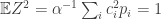
Moreover, for any $p \geq 1$ , using Jensen inequality and the definition of the $c_i$ ,

$\mathbb E |Z|^p = \alpha^{-p/2}\,\sum_i |c_i|^p p_i \leq \alpha^{-p/2}\,\sum_i \mathbb E[|X|^p|\mathcal P_i]\, p_i \leq \alpha^{-p/2}\,\mathbb E |X|^p.$

Therefore, by definition of the sub-Gaussian norm above, we find

$\|Z\|_{\psi_2} = \|\mathcal Q(X)\|_{\psi_2} \leq \|X\|_{\psi_2}/\sqrt{\alpha},$

which shows that $Z = \mathcal Q(X)$ is also sub-Gaussian!

For instance, for a Gaussian rv $X$ , taking $\mathcal{P} = \{(-\infty, 0], (0, +\infty)\}$ , leads to $\mathcal C = \{\pm 1\}$ and $p_0 = p_1 = 1/2$ , since $\mathbb E|X| = \sqrt{2/\pi} = 2 |c_i|$ and $\alpha = 1/2\pi$ . We recover then, by quantization, a Bernoulli rv!

In consequence, a matrix 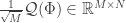$\tfrac{1}{\sqrt M}\mathcal Q(\Phi) \in \mathbb R^{M \times N}$ obtained by quantizing the entries of a random Gaussian matrix $\Phi$ will satisfy, whp, the RIP of order $K$ (as for $\tfrac{1}{\sqrt M} \Phi$ ) provided $M \gtrsim K \log N/K$ , where the hidden constant depends only on $\alpha$ (and implicitly on the quantizing partition $\mathcal P$ ).

From what is described above, it is clear that the entries of $\mathcal Q(\Phi)$ are iid as $\mathcal Q(X)$ with $X \sim \mathcal N(0,1)$ . Then, as explained in [1, 4, 3], it remains to show that the rows of $\mathcal Q(\Phi)$ are isotropic, i.e., that for any row $r$ of $\mathcal Q(\Phi)$ , $\mathbb E(r^T x)^2 = \|x\|^2$ for any vector $x \in \mathbb R^N$ . This trivially holds as $r$ is composed of $N$ entries iid as $Z$ that has unit variance.

Note that nowhere above we have used the Gaussianity of $X$ . Therefore the whole development still holds if we quantify a random matrix whose entries are generated by a sub-Gaussian distribution, possibility already discrete or quantized. In other words, the class of sub-Gaussian random matrices (with iid entries) that are RIP with high probability is somehow closed under entrywise quantization.

Open question:

What will happen if we quantize a structured random matrix, such as a random Fourier ensemble [2], a spreadspectrum sensing matrix [7] or a random convolution [6]? Or more simply random matrices were only the rows (or the columns) are guaranteed to be independent [1]? Do we recover (almost) known random matrix construction such as random partial Hadamard ensembles ?

References:

[1] R. Vershynin, “Introduction to the non-asymptotic analysis of random matrices”, http://arxiv.org/abs/1011.3027

[2] S. Foucart, H. Rauhut. A mathematical introduction to compressive sensing. Vol. 1. No. 3. Basel: Birkhäuser, 2013.

[3] R. Baraniuk, M. Davenport, R. DeVore, M. Wakin, “A simple proof of the restricted isometry property for random matrices”. Constructive Approximation, 28(3), 253-263, 2008.

[4] S. Mendelson, A. Pajor, N. Tomczak-Jaegermann, “Uniform uncertainty principle for bernoulli and subgaussian ensembles. Constructive Approximation, 28(3):277-289, 2008.

[5] R. M. Gray, D. L. Neuhoff, “Quantization”, IEEE Transactions on Information Theory, 44(6), 2325-2383, 1998.

[6] J. Romberg, “Compressive sensing by random convolution”. SIAM Journal on Imaging Sciences, 2(4), 1098-1128, 2009.

[7] G. Puy, P. Vandergheynst, R. Gribonval, Y. Wiaux, “Universal and efficient compressed sensing by spread spectrum and application to realistic Fourier imaging techniques”, EURASIP Journal on Advances in Signal Processing, 2012(1), 1-13.

Quasi-isometric embeddings of vector sets with quantized sub-Gaussian projections

Last January, I was honored to be invited in RWTH Aachen University by Holger Rauhut and Sjoerd Dirksen to give a talk on the general topic of quantized compressed sensing. In particular, I decided to focus my presentation on the quasi-isometric embeddings arising in 1-bit compressed sensing, as developed by a few researchers in this field (e.g., Petros Boufounos, Richard Baraniuk, Yaniv Plan, Roman Vershynin and myself).

In comparison with isometric (bi-Lipschitz) embeddings suffering only from a multiplicative distortion, as for the restricted isometry property (RIP) for sparse vectors sets or Johnson-Lindenstrauss Lemma for finite sets, a quasi-isometric embedding $\bf E: \mathcal K \to \mathcal L$ between two metric spaces $(\mathcal K, d_{\mathcal K})$ and $(\mathcal L,d_{\mathcal L})$ is characterized by both a multiplicative and an additive distortion, i.e., for some values $\Delta_{\oplus},\Delta_{\otimes}>0$ , $\bf E$ respects

$(1- \Delta_{\otimes}) d_{\mathcal K}(\boldsymbol u, \boldsymbol v) - \Delta_\oplus\leq d_{\mathcal L}(\bf E(\boldsymbol u), \bf E(\boldsymbol v)) \leq (1 + \Delta_{\otimes}) d_{\mathcal K}(\boldsymbol u, \boldsymbol v)+\Delta_\oplus,$

for all $\boldsymbol u,\boldsymbol v \in \mathcal K$ .

In the case of 1-bit Compressed Sensing, one observes a quasi-isometric relation between the angular distance of two vectors (or signals) in $\mathbb R^N$ and the Hamming distance of their 1-bit quantized projections in $\{\pm 1\}^M$ . This mapping is simply obtained by keeping the sign (componentwise) of their multiplication by a $M\times N$ random Gaussian matrix. Mathematically,

$\boldsymbol A_{\rm 1bit}: \boldsymbol u \in \mathbb R^N \mapsto \boldsymbol A_{\rm 1bit}(\boldsymbol u) := {\rm sign}(\boldsymbol\Phi\boldsymbol u),$

with $\boldsymbol \Phi \in \mathbb R^{M\times N}$ and $\Phi_{ij} \sim_{\rm iid} \mathcal N(0,1)$ . Notice that for a general sensing matrix (e.g., possibly non-Gaussian), if reachable, ${\bf A}_{1bit}$ can only induce a quasi-isometric relation. This is due to the information loss induced by the “sign” quantization in, e.g., the loss of the signal amplitude. Moreover, it is known that for a Bernoulli sensing matrix $\boldsymbol \Phi \in \{\pm 1\}^{M \times N}$ , two vectors can be arbitrarily close and share the same quantization point [2,5].

Interestingly, it has been shown in a few works that quasi-isometric 1-bit embeddings exist for $K$ -sparse signals [1] or for any bounded subset $\mathcal K$ of $\mathbb R^N$ provided the typical dimension of this set is bounded [2]. This dimension is nothing but the Gaussian mean width $w(\mathcal K)$ of the set [2] defined by

$w(\mathcal K) = \mathbb E \sup_{\boldsymbol u \in \mathcal K} |\boldsymbol g^T \boldsymbol u|,\quad \boldsymbol g \sim \mathcal N(0,{\rm Id}_N).$

Since the 80’s, this dimension has been recognized as central for instance in characterizing random processes [9], shrinkage estimators in signal denoising and high-dimensional statistics [10], linear inverse problem solving with convex optimization [11] or classification efficiency in randomly projected signal sets [12]. Moreover, for the set of bounded K-sparse signals, we have $w(\mathcal K)^2 \leq C K \log N/K$ , which is the quantity of interest for characterizing the RIP of order $K$ of random Gaussian matrices (with other interesting characterizations for the compressible signals set or for “signals” consisting of rank-r matrices).

In [2], by connecting the problem to the context of random tessellation of the sphere $\mathbb S^{N-1}$ , the authors have shown that if $M$ is larger than

$M \geq C \epsilon^{-6} w(\mathcal K)^2,$

then, for all $x,y \in \mathcal K$ ,

$d_{\rm ang}(x,y) - \epsilon \leq d_H(\boldsymbol A_{\rm 1bit}(x), \boldsymbol A_{\rm 1bit}(y)) \leq d_{\rm ang}(x,y) + \epsilon.$

For $K$ -sparse vectors, this condition is even reduced to $M=O(\epsilon^{-2} K \log N/K)$ as shown in [1].

As explained in my previous post on quantized embedding and the funny connection with Buffon’s needle problem, I have recently noticed that for finite sets $\mathcal K \subset \mathbb R^N$ , quasi-isometric relations also exist with high probability between the Euclidean distance (or $\ell_2$ -distance) of vectors and the $\ell_1$ -distance of their (dithered) quantized random projections. Generalizing ${\bf A}_{\rm 1bit}$ above, this new mapping reads

${\bf A}: \boldsymbol u \in \mathbb R^N \mapsto \mathcal {\bf A}(\boldsymbol u) := Q(\boldsymbol \Phi\boldsymbol u + \boldsymbol \xi) \in \delta \mathbb Z^M,$

for a (“round-off”) scalar quantizer $\mathcal Q(\cdot) = \delta \lfloor \cdot / \delta \rfloor$ with resolution $\delta>0$ applied componentwize on vectors, a random Gaussian $\boldsymbol \Phi$ (as above) and a dithering $\boldsymbol \xi \in \mathbb R^{M}$ , with $\xi_i \sim_{\rm iid} \mathcal U([0, \delta])$ uniformizing the action of the quantizer (as used in [6] for more general quantizers).

In particular, provided $M \geq C \epsilon^{-2}\log |\mathcal K|$ , with high probability, for all $\boldsymbol x, \boldsymbol y \in \mathcal K$ ,

$(\sqrt{\frac{2}{\pi}} - \epsilon)\,\|\boldsymbol x - \boldsymbol y\| - c\delta\epsilon \leq \frac{1}{M}\|\boldsymbol A(\boldsymbol x) - \boldsymbol A(\boldsymbol y)\|_1 \leq (\sqrt{\frac{2}{\pi}}+\epsilon)\,\|\boldsymbol x - \boldsymbol y\| + c\delta\epsilon,\qquad(1)$

for some general constants $C,c>0$ .

One observes that the additive distortion of this last relation reads $\Delta_\oplus = c\delta\epsilon$ , i.e., it can be made arbitrarily low with $\epsilon$ ! However, directly integrating the quantization in the RIP satisfied by $\boldsymbol \Phi$ would have rather led to a constant additive distortion, only function of $\delta$ .

Remark: For information, as provided by an anonymous expert reviewer, it happens that a much shorter and elegant proof of this fact exists using the sub-Gaussian properties of the quantized mapping $\bf A$ (see Appendix A in the associated revised paper).

In that work, the question remained, however, on how to extend (1) for vectors taken in any (bounded) subset $\mathcal K$ of $\mathbb R^N$ , hence generalizing the quasi-isometric embeddings observed for 1-bit random projections? Moreover, it was still unclear if the sensing matrix $\boldsymbol \Phi$ could be non-Gaussian, i.e., if any sub-Gaussian matrix (e.g., Bernoulli $\pm 1$ ) could define a suitable $\bf A.$

While I was in Aachen discussing with Holger and Sjoerd during and after my presentation, I realized that the works [2-5] of Plan, Verhsynin, Ai and collaborators provided already many important tools whose adaptation to the mapping $\bf A$ above could answer those questions.

At the heart of [2] lies the equivalence between $d_H(\boldsymbol A_{\rm 1bit}(\boldsymbol x), \boldsymbol A_{\rm 1bit}(\boldsymbol y))$ and a counting procedure associated to

$d_H(\boldsymbol A_{\rm 1bit}(\boldsymbol x), \boldsymbol A_{\rm 1bit}(\boldsymbol y)) = \frac{1}{M} \sum_i \mathbb I[\mathcal E (\boldsymbol \varphi_i^T \boldsymbol x, \boldsymbol \varphi_i^T \boldsymbol y)],$

where $\boldsymbol \varphi_i$ is the $i^{\rm th}$ row of $\boldsymbol \Phi$ , $\mathbb I(A)$ is the indicator set function equals to 1 if $A$ is non-empty and 0 otherwise, and

$\mathcal E(a,b) = \{{\rm sign}(a) \neq {\rm sign}(b)\}$ .

In words, $d_H(\boldsymbol A_{\rm 1bit}(\boldsymbol x), \boldsymbol A_{\rm 1bit}(\boldsymbol y))$ counts the number of hyperplanes defined by the normals $\boldsymbol \varphi_i$ that separate $\boldsymbol x$ from $\boldsymbol y$ .

Without giving too many details in this post, the work [2] leverages this equivalence to make a connection with tessellation of the $(N-1)$ -sphere where it is shown that the number of such separating random hyperplanes is somehow close (up to some distortions) to the angular distance between the two vecors. They obtain this by “softening” the Hamming distance above, i.e., by introducing, for some $t \in \mathbb R$ , the soft Hamming distance

$d^t_H(\boldsymbol A_{\rm 1bit}(\boldsymbol x), \boldsymbol A_{\rm 1bit}(\boldsymbol y)) := \frac{1}{M} \sum_i \mathbb I[\mathcal F^t(\boldsymbol \varphi_i^T \boldsymbol x, \boldsymbol \varphi_i^T \boldsymbol y)],$

with now

$\mathcal F^t(a,b) = \{a > t, b \leq -t\} \cup \{a \leq -t, b > t\}$ .

This distance has an interesting continuity property compared to $d_H = d^0_H$ . In particular, if one allows $t$ to vary, it is continuous up to small ( $\ell_1$ ) perturbations of $\boldsymbol x$ and $\boldsymbol y$ .

In our context, considering the quantized mapping $\bf A$ specified above, we can define the generalized soften distance :

$\mathcal Q^t(\boldsymbol x,\boldsymbol y) := \tfrac{\delta}{M}\,\sum_{i=1}^M \sum_{k\in\mathbb Z} \mathbb I[\mathcal F^t(\boldsymbol \varphi_i^T \boldsymbol x + \xi_i - k\delta, \boldsymbol \varphi_i^T \boldsymbol y + \xi_i - k\delta)].$

When $t=0$ we actually recover the distance used in the quasi-isometry (1), i.e.,

$\mathcal Q^0(\boldsymbol x,\boldsymbol y) = \frac{1}{M} \|\boldsymbol A(\boldsymbol x) - \boldsymbol A(\boldsymbol y)\|_1,$

similarly to the recovering of the Hamming distance in 1-bit case.

The interpretation of $\mathcal Q^t(\boldsymbol x,\boldsymbol y)$ when $t=0$ is now that we again count the number of hyperplanes defined by the normals $\boldsymbol \varphi_i$ that separate $\boldsymbol x$ from $\boldsymbol y$ , but now, for each measurement index $1 \leq i \leq M$ this count can be bigger than 1 as we allow multiple parallel hyperplanes for each normal $\boldsymbol \varphi_i$ , all $\delta$ far apart. This is in connection with the “hyperplane wave partitions” defined in [7,8], e.g., for explaining quantization of vector frame coefficients. As explained in the paper, when $t\neq 0$ , then $\mathcal Q^t$ relaxes (for $t < 0$ ) or strengthens (for $t \geq 0$ ) the conditions allowing to count a separating hyperplane.

As for 1-bit projections, we can show the continuity of $\mathcal Q^t(\boldsymbol x,\boldsymbol y)$ with respect to small ( $\ell_2$ now) perturbation of $\boldsymbol x$ and $\boldsymbol y$ , and this fact allows to study the random (sub-Gaussian) concentration of $\mathcal Q^t(\boldsymbol x,\boldsymbol y)$ , i.e., studying it for a coverage of the set of interest, and then extending it to the whole set from this continuity.

From this observation, and after a few months of works, I have gathered all these developments in the following paper, now submitted on arxiv:

“Small width, low distortions: Quasi-isometric embeddings
with quantized sub-Gaussian random projections”, arXiv:1504.06170

Briefly, benefiting of the context defined above, this work contains two main results.

First, it shows that given a symmetric sub-Gaussian distribution $\varphi$ and a precision $\epsilon > 0$ , if

$M \geq C \epsilon^{-5} w(\mathcal K)^2$

and if the sensing matrix $\boldsymbol \Phi$ has entries i.i.d. as $\varphi$ , then, with high probability, the mapping $\bf A$ above provides a $\ell_2/\ell_1$ -quasi-isometry between vector pair of $\mathcal K$ whose difference are “not too sparse” (as already noticed in [5] for 1-bit CS) and their images in $\delta \mathbb Z^M$ . More precisely, for some $c >0$ , if for $K_0 >0$ ,

$\boldsymbol x - \boldsymbol y \in C_{K_0} = \{\boldsymbol u \in \mathbb R^N: K_0\|\boldsymbol u\|^2_\infty \leq \|\boldsymbol u\|^2\}$

then, given some constant $\kappa_{\rm sg}$ depending on the sub-Gaussian distribution $\varphi$ (with $\kappa_{\rm sg} = 0$ if $\varphi$ is Gaussian),

${(\sqrt{\frac{2}{\pi}} - \epsilon - \frac{\kappa_{\rm sg}}{\sqrt K_0}) \|\boldsymbol x - \boldsymbol y\|- c\epsilon\delta\ \leq\ \frac{1}{M} \|\boldsymbol A(\boldsymbol x) - \boldsymbol A(\boldsymbol y)\|_1\ \leq\ (\sqrt{\frac{2}{\pi}} + \epsilon + \frac{\kappa_{\rm sg}}{\sqrt K_0}) \|\boldsymbol x - \boldsymbol y\|+ c\epsilon\delta.}$

Interestingly, in this quasi-isometric embedding, we notice that the additive distortion is driven by $\epsilon\delta$ as in (1) while the multiplicative distortion reads now

$\Delta_{\otimes} = \epsilon + \frac{\kappa_{\rm sg}}{\sqrt K_0}$

In addition to its common dependence in the precision $\epsilon$ , this distortion is also function of the “antisparse” nature of $\boldsymbol x - \boldsymbol y$ . Indeed, if $\boldsymbol u \in C_{K_0}$ then it cannot be sparser than $K_0$ with anyway $C_{K_0} \neq \mathbb R^N \setminus \Sigma_{K_0}$ . In other words, when the matrix $\boldsymbol \Phi$ is non-Gaussian (but sub-Gaussian anyway), the distortion is smaller for “anti-sparse” vector differences.

In the particular case where $\mathcal K$ is the set of bounded $K$ -sparse vectors in any orthonormal basis, then only

$M \geq C \epsilon^{-2} \log(c N/K\epsilon^{3/2})$

measurements suffice for defining the same embedding with high probability. As explained in the paper, this case allows somehow to mitigate the anti-sparse requirement as sparse vectors in some basis can be made less sparse in another, e.g., for dual bases such as DCT/Canonical, Noiselet/Haar, etc.

The second result concerns the consistency width of the mapping $A$ , i.e., the biggest distance separating distinct vectors that are projected by $A$ on the same quantization point. With high probability, it happens that the consistency width $\epsilon$ of any pair of vectors whose difference is again“not too sparse” decays as

$\epsilon = O(M^{-1/4}\,w(\mathcal K)^{1/2})$

for a general subset $\mathcal K$ and, up to some log factors, as $\epsilon = M^{-1}$ for sparse vector sets.

Open problem: I’m now wondering if the tools and results above could be extended to other quantizers $\mathcal Q$ , such as the universal quantizer defined in [6]. This periodic quantizer has been shown to provide exponentially decaying distortions [6,13] for embedding of sparse vectors, with interesting applications (e.g., information retrieval). Knowing if this holds for other vector sets and for other (sub-Gaussian) sensing matrix is an appealing open question.

References:

[1] L. Jacques, J. N. Laska, P. T. Boufounos, and R. G Baraniuk. “Robust 1-bit compressive sensing via binary
stable embeddings of sparse vectors”. IEEE Transactions on Information Theory, 59(4):2082–2102, 2013.

[2] Y. Plan and R. Vershynin. “Dimension reduction by random hyperplane tessellations”. Discrete & Computational Geometry, 51(2):438–461, 2014, Springer.

[3] Y. Plan and R. Vershynin. “Robust 1-bit compressed sensing and sparse logistic regression: A convex programming approach”. IEEE Transactions on Information Theory, 59(1): 482–494, 2013.

[4] Y. Plan and R. Vershynin. “One-bit compressed sensing by linear programming”. Communications on Pure and Applied Mathematics, 66(8):1275–1297, 2013.

[5] A. Ai, A. Lapanowski, Y. Plan, and R. Vershynin. “One-bit compressed sensing with non-gaussian measurements”. Linear Algebra and its Applications, 441:222–239, 2014.

[6] P. T. Boufounos. Universal rate-efficient scalar quantization. IEEE Trans. Info. Theory, 58(3):1861–1872, March 2012.

[7] V. K Goyal, M. Vetterli, and N. T. Thao. Quantized overcomplete expansions in $\mathbb R^N$ : Analysis, synthesis, and algorithms. IEEE Trans. Info. Theory, 44(1):16–31, 1998.

[8] N. T . Thao and M. Vetterli. “Lower bound on the mean-squared error in oversampled quantization of periodic signals using vector quantization analysis”. IEEE Trans. Info. Theory, 42(2):469–479, March 1996.

[9] A. W. Vaart and J. A. Wellner. Weak convergence and empirical processes. Springer, 1996.

[10] V. Chandrasekaran and M. I. Jordan. Computational and statistical tradeoffs via convex relaxation. arXiv preprint arXiv:1211.1073, 2012.

[11] V. Chandrasekaran, B. Recht, P. A Parrilo, and A. S. Willsky. The convex geometry of linear inverse problems. Foundations of Computational mathematics, 12(6):805–849, 2012.

[12] A. Bandeira, D. G Mixon, and B. Recht. Compressive classification and the rare eclipse problem. arXiv preprint arXiv:1404.3203, 2014.

[13] P. T. Boufounos and S. Rane. Efficient coding of signal distances using universal quantized embeddings. In Proc. Data Compression Conference (DCC), Snowbird, UT, March 20-22 2013.

Testing a Quasi-Isometric Quantized Embedding

It took me a certain time to do it. Here is at least a first attempt to test numerically the validity of some of the results I obtained in “A Quantized Johnson Lindenstrauss Lemma: The Finding of Buffon’s Needle” (arXiv)

I have decided to avoid using the too conventional matlab environment. Rather, I took this exercise as an opportunity to learn the “ipython notebooks” and the wonderful tools provided by the SciPy python ecosystem.

In short, for those of you who don’t know it, the ipython notebooks allow you to generate actual scientific HTML reports with (latex rendered) explanations and graphics.

The result cannot be properly presented on this blog (hosted on WordPress), so, I decided to share the report through IPython Notebook Viewer website.
Here it is:

“Testing a Quasi-Isometric Embedding”

(update 21/11/2013) … and a variant of it estimating a “curve of failure” (rather than playing with standard deviation analysis):

“Testing a Quasi-Isometric Embedding with Percentile Analysis”

Moreover, on these two links, you have also the possibility to download the corresponding script for running it on your own IPython notebook system.

If you have any comments or corrections, don’t hesitate to add them below in the “comment” section. Enjoy!

When Buffon’s needle problem meets the Johnson-Lindenstrauss Lemma

(left) Picture of [8, page 147] stating the initial formulation of Buffon’s needle problem (Courtesy of E. Kowalski’s blog) (right) Scheme of Buffon’s needle problem.

(This post is related to a paper entitled “A Quantized Johnson Lindenstrauss Lemma: The Finding of Buffon’s Needle” (arxiv, pdf) that I have recently submitted for publication.)

Last July, I read the biography of Paul Erdős written by Paul Hoffman and entitled “The Man Who Loved Only Numbers“. This is really a wonderful book sprinkled with many anecdotes about the particular life of this great mathematician and about his appealing mathematical obsessions (including prime numbers).

At one location of this book my attention was caught by the mention of what is called the “Buffon’s needle problem”. It seems to be a very old and well-known problem in the field of “geometrical probability” and I discovered later that Emmanuel Kowalski (Math dep., ETH Zürich, Switzerland) explained it in one of his blog posts.

In short, this problem, formulated by Georges-Louis Leclerc, Comte de Buffon in France in one of the numerous volumes of his impressive work entitled “L’Histoire Naturelle”, is formulated as follows:

“I suppose that in a room where the floor is simply divided by parallel joints one throws a stick (N/A: later called “needle”) in the air, and that one of the players bets that the stick will not cross any of the parallels on the floor, and that the other in contrast bets that the stick will cross some of these parallels; one asks for the chances of these two players.”

The English translation is due to [1]. The solution (published by Leclerc in 1777) is astonishingly simple: for a short needle compared to the separation $\delta$ between two consecutive parallels, the probability of having one intersection between the needle and the parallels is equal to the needle length times $\frac{1}{\pi\delta}$ ! If the needle is longer, then this probability is less easy to express but the expectation of the number of intersections (which can now be bigger than one) remains equal to this value. Surprisingly, this result still holds if the needle is replaced by a finite smooth curve that some authors then call the “noodle” problem (e.g., in [5])

The reason why this problem rang a bell is related to its similarity with a quantization process!

Indeed, think for a while to the needle as the segment formed by two points $\boldsymbol x,\boldsymbol y$ in the plane $\mathbb R^2$ and assume all the parallel joints normal to the first canonical axis $\boldsymbol e_1$ of $\mathbb R^2$ . Let us also think to the area defined by two consecutive joints as an infinite strip of width $\delta$ . Then, the number of intersections that this “needle” makes with the grid of parallel joints is related to the distance between the two strips occupied by the two points, i.e., to the distance between a uniform quantization (or rounding off) of the $\boldsymbol e_1$ -coordinate of the two points!

From this observation, if I realized that if we randomly turn these two points with a random rotation $\boldsymbol R$ of $SO(2)$ and if a random translation $u$ along the $e_1$ -axis is added to their coordinates, the context of the initial Buffon’s problem is exactly recovered!

Interestingly enough, after this randomized transformation, the first coordinate of one of the two points (defining the needle extremities), say $\boldsymbol x$ , reads

$\boldsymbol e_1^T (\boldsymbol R \boldsymbol x + u \boldsymbol e_1) = (\boldsymbol R^T \boldsymbol e_1)^T \boldsymbol x + u\quad \sim\quad \boldsymbol \theta^T \boldsymbol x + u$

where $\boldsymbol \theta$ is a uniform random variable on the circle $\mathbb S^1 \subset \mathbb R^2$ . What you observe on the right of the last equivalence is nothing but a random projection of the point $\boldsymbol x$ on the direction $\boldsymbol \theta \in \mathbb S^1$ .

This was really amazing to discover: after these very simple developments, I had in front of me a kind of triple equivalence between Buffon’s needle problem, quantization process in the plane and a well-known linear random projection procedure. This boded well for a possible extension of this context to high-dimensional (random) projection procedures, e.g., those used in common linear dimensionality reduction methods and in the compressed sensing theory.

Actually, this gave me a new point of view for solving these two connected questions: How to combine the well-known Johnson-Lindenstrauss Lemma with a quantization of the embedding it proposes? What (new) distortion of the embedding can we expect from this non-linear operation?

Let me recall the tenet of the JL Lemma: For a set $\mathcal S \subset \mathbb R^N$ of $S$ points, if you fix $0<\epsilon<1$ and $\delta >0$ , as soon as $M > M_0 = O(\epsilon^{-2}\log S)$ , there exist a mapping $\boldsymbol f:\mathbb R^N\to \mathbb R^M$ such that, for all pairs $\boldsymbol u,\boldsymbol v\in \mathcal S$ ,

with some possible variants on the selected norms, e.g., from some measure concentration results in Banach space [6], the result is still true with the same condition on $M$ if we take the $\ell_1$ norm of $\boldsymbol f(\boldsymbol u) - \boldsymbol f(\boldsymbol v)$ . This is this variant that matters in the rest of this post.

It took me some while but after having generalized Buffon’s needle problem to a $N$ -dimensional space (where the needle is still a 1-D segment “thrown” randomly in a grid of $(N-1)$ -dimensional parallel hyperplane that are $\delta>0$ apart) — which provided a few interesting asymptotic relations concerning this probabilistic problem — I was also able to generalize the previous equivalence as follows: Uniformly quantizing the random projections in $\mathbb R^M$ of two points in $\mathbb R^N$ and measuring the difference between their quantized values is fully equivalent to study the number of intersections made by the segment determined by those two points (seen as a Buffon’s needle) with a parallel grid of $(N-1)$ -dimensional hyperplanes.

This equivalence was the starting point to discover the following proposition (the main result of the paper referenced above) which can be seen as a quantized form of the Johnson-Lindenstrauss Lemma:

Let $\mathcal S \subset \mathbb R^N$ be a set of $S$ points. Fix $0<\epsilon<1$ and $\delta >0$ . For $M > M_0 = O(\epsilon^{-2}\log S)$ , there exist a non-linear mapping $\boldsymbol \psi:\mathbb R^N\to \mathbb (\delta Z)^M$ and two constants $c,c'>0$ such that, for all pairs $\boldsymbol u,\boldsymbol v\in \mathcal S$ ,

$(1 - \epsilon)\,\|\boldsymbol u - \boldsymbol v\|\,-\,c\,\delta\,\epsilon\ \leq\ \frac{c'}{M} \|\boldsymbol \psi(\boldsymbol u)-\boldsymbol \psi(\boldsymbol v)\|_1 \ \leq\ (1 + \epsilon)\|\boldsymbol u-\boldsymbol v\|\,+\,c\,\delta\,\epsilon.$

Moreover, this mapping $\boldsymbol \psi$ can be randomly constructed by

$\boldsymbol \psi(\boldsymbol u) = \mathcal Q_{\delta}(\boldsymbol \Phi \boldsymbol u + \boldsymbol \xi),$

where $\mathcal Q$ is a uniform quantization of bin width $\delta>0$ , $\boldsymbol \Phi$ is a $M \times N$ Gaussian random matrix and $\boldsymbol \xi$ is a uniform random vector over $[0, \delta]^M$ . Except for the quantization, this construction is similar to the one introduced in [7] (for non-regular quantizers).

Without entering into the details, the explanation of this result comes from the fact that the random projection $\boldsymbol \Phi$ can be seen as a random rotation of $\mathbb R^N$ followed by a random scaling of the vector amplitude. Therefore, conditionally to this amplitude, the equivalence with Buffon’s problem is recovered for a (scaled) needle determined by the vectors $\boldsymbol u$ and $\boldsymbol v$ above, the dithering $\boldsymbol \xi$ playing the role of the random needle shift.

Interestingly, compared to the common JL Lemma, the mapping is now “quasi-isometric“: we observe both an additive and a multiplicative distortions on the embedded distances of $\boldsymbol u, \boldsymbol v \in \mathcal S$ . These two distortions, however, decay as
$O(\sqrt{\log S/M})$ when $M$ increases!

This kind additive distortion decay was already observed for “binary” (or one-bit) quantization procedure [2, 3, 4] applied on random projection of points (e.g., for 1-bit compressed sensing). Above, we still observe such a distortion for the (multi-bit) quantization above and, moreover, this distortion is combined with a multiplicative one while both decay when $M$ increases. This fact is new, to the best of my knowledge.

Moreover, for coarse quantization, i.e., for high $\delta$ compared to
the typical size of $\mathcal S$ , the distortion is mainly additive, while for small $\delta$ we tend to a classical Lipschitz isometric embedding, as provided by the JL Lemma.

Interested blog reader can have a look to my paper for a clearer (I hope) presentation of this informal summary. His summary is as follows:

“In 1733, Georges-Louis Leclerc, Comte de Buffon in France, set the ground of geometric probability theory by defining an enlightening problem: What is the probability that a needle thrown randomly on a ground made of equispaced parallel strips lies on two of them? In this work, we show that the solution to this problem, and its generalization to $N$ dimensions, allows us to discover a quantized form of the Johnson-Lindenstrauss (JL) Lemma, i.e., one that combines a linear dimensionality reduction procedure with a uniform quantization of precision $\delta>0$ . In particular, given a finite set $\mathcal S \subset \mathbb R^N$ of $S$ points and a distortion level $\epsilon>0$ , as soon as $M > M_0 = O(\epsilon^{-2} \log S)$ , we can (randomly) construct a mapping from $(\mathcal S, \ell_2)$ to $(\,(\delta\,\mathbb Z)^M, \ell_1)$ that approximately preserves the pairwise distances between the points of $\mathcal S$ . Interestingly, compared to the common JL Lemma, the mapping is quasi-isometric and we observe both an additive and a multiplicative distortions on the embedded distances. These two distortions, however, decay as $O(\sqrt{\log S/M})$ when $M$ increases. Moreover, for coarse quantization, i.e., for high $\delta$ compared to the set radius, the distortion is mainly additive, while for small $\delta$ we tend to a Lipschitz isometric embedding. Finally, we show that there exists “almost” a quasi-isometric embedding of $(\mathcal S, \ell_2)$ in $( (\delta \mathbb Z)^M, \ell_2)$ . This one involves a non-linear distortion of the $\ell_2$ -distance in $\mathcal S$ that vanishes for distant points in this set. Noticeably, the additive distortion in this case is slower and decays as $O((\log S/M)^{1/4})$ .”

Hoping there is no killing bug in my developments, any comments are also welcome.

References:

[1] J. D. Hey, T. M. Neugebauer, and C. M. Pasca, “Georges-Louis Leclerc de Buffons Essays on Moral Arithmetic,” in The Selten School of Behavioral Economics, pp. 245–282. Springer, 2010.

[2] L. Jacques, J. N. Laska, P. T. Boufounos, and R. G. Baraniuk, “Robust 1-Bit Compressive Sensing via Binary Stable Embeddings of Sparse Vectors,” IEEE Transactions on Information Theory, Vol. 59(4), pp. 2082-2102, 2013.

[3] Y. Plan and R. Vershynin, “One-bit compressed sensing by linear programming,” Communications on Pure and Applied Mathematics, to appear. arXiv:1109.4299, 2011.

[4] M. Goemans and D. Williamson, “Improved approximation algorithms for maximum cut and satisfiability problems using semidefinite programming,” Journ. ACM, vol. 42, no. 6, pp. 1145, 1995.

[5] J. F. Ramaley, “Buffon’s noodle problem,” The American Mathematical Monthly, vol. 76, no. 8, pp. 916–918, 1969.

[6] M. Ledoux and M. Talagrand, Probability in Banach Spaces: Isoperimetry and Processes, Springer, 1991.

[7] P. T. Boufounos, “Universal rate-efficient scalar quantization.” Information Theory, IEEE Transactions on 58.3 (2012): 1861-1872.

[8] G. C. Buffon, “Essai d’arithmetique morale,” Supplément à l’histoire naturelle, vol. 4, 1777. See also: http://www. buffon.cnrs.fr

Recovering sparse signals from sparsely corrupted compressed measurements

Last Thursday after an email discussion with Thomas Arildsen, I was thinking again to the nice embedding properties discovered by Y. Plan and R. Vershynin in the context of 1-bit compressed sensing (CS) [1].

I was wondering if these could help in showing that a simple variant of basis pursuit denoising using a $\ell_1$ -fidelity constraint, i.e., a $\ell_1/\ell_1$ solver, is optimal in recovering sparse signals from sparsely corrupted compressed measurements. After all, one of the key ingredient in 1-bit CS is the $\rm sign$ operator that is, interestingly, the (sub) gradient of the $\ell_1$ -norm, and for which many random embedding properties have been recently proved [1,2,4].

The answer seems to be positive when you merge these results with the simplified BPDN optimality proof of E. Candès [3]. I have gathered these developments in a very short technical report on arXiv:

Laurent Jacques, “On the optimality of a L1/L1 solver for sparse signal recovery from sparsely corrupted compressive measurements” (Submitted on 20 Mar 2013)
Abstract: This short note proves the $\ell_2-\ell_1$ instance optimality of a $\ell_1/\ell_1$ solver, i.e., a variant of basis pursuit denoising with a $\ell_1$ -fidelity constraint, when applied to the estimation of sparse (or compressible) signals observed by sparsely corrupted compressive measurements. The approach simply combines two known results due to Y. Plan, R. Vershynin and E. Candès.

Briefly, in the context where a sparse or compressible signal $\boldsymbol x \in \mathbb R^N$ is observed by a random Gaussian matrix $\boldsymbol \Phi \in \mathbb R^{M\times N}$ , i.e., with $\Phi_{ij} \sim_{\rm iid} \mathcal N(0,1)$ , according to the noisy sensing model

$\boldsymbol y = \boldsymbol \Phi \boldsymbol x + \boldsymbol n, \qquad (1)$ ,

where $\boldsymbol n$ is a “sparse” noise with bounded $\ell_1$ -norm $\|\boldsymbol n\|_1 \leq \epsilon$ ( $\epsilon >0$ ), the main point of this note is to show that the $\ell_1/\ell_1$ program

$\boldsymbol x^* = {\rm arg min}_{\boldsymbol u} \|\boldsymbol u\|_1 \ {\rm s.t.}\ \| \boldsymbol y - \boldsymbol \Phi \boldsymbol u\|_1\qquad ({\rm BPDN}-\ell_1)$

provides, under certain conditions, a bounded reconstruction error (aka $\ell_2-\ell_1$ – instance optimal):

Noticeably, the two conditions (2) and (3) are not unrealistic, I mean, they are not worst than assuming the common restricted isometry property ;-). Indeed, thanks to [1,2], we can show that they hold for random Gaussian matrices as soon as $M = O(\delta^{-6} K \log N/K)$ :

As explained in the note, it seems also that the dependency in $\delta^{-6}$ can be improved to $\delta^{-2}$ for having (5). The question of proving the same dependence for (6) is open. You’ll find more details (and proofs) in the note.

Comments are of course welcome

References:
[1] Y. Plan and R. Vershynin, “Robust 1-bit compressed sensing and sparse logistic regression: A convex programming approach,” IEEE Transactions on Information Theory, to appear., 2012.

[2] Y. Plan and R. Vershynin, “Dimension reduction by random hyperplane tessellations,” arXiv preprint arXiv:1111.4452, 2011.

[3] E. Candès, “The restricted isometry property and its implications for compressed sensing,” Compte Rendus de l’Academie des Sciences, Paris, Serie I, vol. 346, pp. 589–592, 2008.

[4] L. Jacques, J. N. Laska, P. T. Boufounos, and R. G. Baraniuk, “Robust 1-Bit Compressive Sensing via Binary Stable Embeddings of Sparse Vectors”
IEEE Transactions on Information Theory, in press.

A useless non-RIP Gaussian matrix

Recently, for some unrelated reasons, I discovered that it is actually very easy to generate a Gaussian matrix $\Phi$ that does not respect the restricted isometry property (RIP) [1]. I recall that such a matrix is RIP if there exists a (restricted isometry) constant $0<\delta<1$ such that, for any $K$ -sparse vector $w\in \mathbb R^N$ ,

$(1-\delta)\|w\|^2\leq \|\Phi w\|^2 \leq (1+\delta)\|w\|^2$ .

This is maybe obvious and it probably serves to nothing but here is anyway the argument.

Take a $K$ -sparse vector $x$ in $\mathbb R$ and generate randomly two Gaussian matrices $U$ and $V$ in $\mathbb R^{M\times N}$ with i.i.d. entries drawn from $\mathcal N(0,1)$ . From the vectors $a=Ux$ and $b=Vx$ , you can form two new vectors $c$ and $s$ such that $c_i = a_i / \sqrt{a_i^2 + b_i^2}$ and $s_i = b_i / \sqrt{a_i^2 + b_i^2}$ .

Then, it is easy to show that matrix

$\Phi = {\rm diag}(c) V - {\rm diag}(s)U\qquad(1)$

is actually Gaussian except in the direction of $x$ (where it vanishes to 0).

This can be seen more clearly in the case where $x = (1,0,\,\cdots,0)^T$ . Then the first column of $\Phi$ is $0$ and the rest of the matrix is independent of ${\rm diag}(c)$ and ${\rm diag}(s)$ . Conditionally to the value of these two diagonal matrices, this part of $\Phi$ is therefore Gaussian with each $ij$ entry ( $j\geq 2$ ) of variance $c_i^2 + s_i^2 = 1$ . Then, the condition can be removed by expectation rule to lead to the cdf of $\Phi$ , and then to the pdf by differentiation, recovering the Gaussian distribution in the orthogonal space of $x$ .

However, $\Phi$ cannot be RIP. First, obviously since $\Phi x = 0$ which shows, by construction, that at least one $K$ -sparse vector (that is, $x$ ) is in the null space of $\Phi$ . Second, by taking vectors in $x + \Sigma_K = x + \{u: \|u\|_0 \leq K \}$ , we clearly have $\|\Phi (x + u)\| = \|\Phi u\|$ for any $u \in \Sigma_K$ . Therefore, we can alway take the norm of $u$ sufficiently small so that $\|\Phi (x + u)\|$ is far from $\|x + u\|$ .

Of course, for the space of $K$ -sparse vectors orthogonal to $x$ , the matrix is still RIP. It is easy to follow the argument above for proving that $\Phi$ is Gaussian in this space and then to use classical RIP proof [2].

All this is also very close from the “Cancel-then-Recover” strategy developed in [3]. The only purpose of this post to prove the (useless) result that combining two Gaussian matrices as in (1) leads to a non-RIP matrix.

References:

[1] Candes, Emmanuel J., and Terence Tao. “Decoding by linear programming.” Information Theory, IEEE Transactions on 51.12 (2005): 4203-4215.

[2] Baraniuk, Richard, et al. “A simple proof of the restricted isometry property for random matrices.” Constructive Approximation 28.3 (2008): 253-263.

[3] Davenport, Mark A., et al. “Signal processing with compressive measurements.” Selected Topics in Signal Processing, IEEE Journal of 4.2 (2010): 445-460.

Tomography of the magnetic fields of the Milky Way?

I have just found this “new” (well 150 years old actually) tomographical method… for measuring the magnetic field of our own galaxy

“New all-sky map shows the magnetic fields of the Milky Way with the highest precision“
by Niels Oppermann et al. (arxiv work available here)

Selected excerpt:

“… One way to measure cosmic magnetic fields, which has been known for over 150 years, makes use of an effect known as Faraday rotation. When polarized light passes through a magnetized medium, the plane of polarization rotates. The amount of rotation depends, among other things, on the strength and direction of the magnetic field. Therefore, observing such rotation allows one to investigate the properties of the intervening magnetic fields.”

Mmmm… very interesting, at least for my personal knowledge of the wonderful tomographical problem zoo (amongst gravitational lensing, interferometry, MRI, deflectometry).

P.S. Wow… 16 months without any post here. I’m really bad.

Some comments on Noiselets

Recently, a friend of mine asked me few questions about Noiselets for Compressed Sensing applications, i.e., in order to create efficient sensing matrices incoherent with signal which are sparse in the Haar/Daubechies wavelet basis. It seems that some of the answers are difficult to find on the web (but I’m sure they are well known to specialists) and I have therefore decided to share the ones I got.

Context:

I wrote in 2008 a tiny Matlab toolbox (see here) to convince myself that the Noiselet followed a Cooley-Tukey implementation already followed by the Walsh-Hadamard transform. It should have been optimized in C but I lacked of time to write this.Since this first code, I realized that Justin Romberg wrote already in 2006 with Peter Stobbe a fast code (also O(N log N) but much faster than mine) available here:

http://users.ece.gatech.edu/~justin/spmag

People could be interested in using Justin’s code since, as it will be clarified from my answers given below, it is already adapted to real valued signals, i.e., it produces real valued noiselets coefficients.

Q1. Do we need to use both the real and imaginary parts of noiselets to design sensing matrices (i.e., building the $\Phi$ matrix)? Can we use just the real part or just the imaginary part)? Any reason why you’d do one thing or another?

As for the the Random Fourier Ensemble sensing, what I personally do when I use noiselet sensing is to pick uniformly at random $M/2$ complex values in half the noiselet-frequency domain, and concatenate the real and the imaginary part into a real vector of length $M=2*M/2$ . The adjoint (transposed) operation — often needed in most of Compressed Sensing solvers — must of course sum the previously split real and imaginary parts into $M/2$ complex values before to pad the complementary measured domain with zeros and run the inverse noiselet transform.

To understand the special treatment of the real and the imaginary parts (and not simply by considering it similar to what is done for Random Fourier Ensemble), let us consider the origin, that is, Coifman et al. Noiselets paper.

Recall that in this paper, two kinds of noiselets are defined. The first basis, the common Noiselets basis on the interval $[0, 1]$ , is defined thanks to the recursive formulas:

The second basis, or Dragon Noiselets, is slightly different. Its elements are symmetric under the change of coordinates $x \to 1-x$ . Their recursive definition is

To be more precise, the two sets

$\{f_j: 2^N\leq j < 2^{N+1}\}$ ,

$\{g_j: 2^N\leq j < 2^{N+1}\}$ ,

are orthonormal bases for piecewise constant functions at resolution $2^N$ , that is, for functions of

$V_N = \{h(x): h\ \textrm{is constant over each}\big[2^{-N}k,2^{-N}(k+1)\big), 0\leq k < 2^N \}.$

In Coifman et al. paper, the recursive definition of Eq. (2) (and also Eq (4) for Dragon Noiselets), which connects the noiselet functions between the noiselet index $n$ and indices $2n$ or $2n+1$ , is simply a common butterfly diagram that sustains the Cooley-Tukey implementation of the Noiselet transform.

The coefficients involved in Eqs (2) and (4) are simply $1 \pm i$ , which are of course complex conjugate of each other.

Therefore, in the Noiselet transform $\hat X$ of a real vector $X$ of length $2^N$ (in one to one correspondance with the piecewise constant functions of $V_N$ ) involving the noiselets of indices $n \in \{2^N, ..., 2^{N+1}-1\}$ , the resulting decomposition diagram is fully symmetric (with a complex conjugation) under a flip of indices $k \leftrightarrow k' = 2^N - 1 - k$ , for $k = 0,\, \cdots, 2^N -1$ .

This shows that

$\hat X_k = \hat X^*_{k'}$ ,

with ${(\cdot)}^*$ the complex conjugation, if $X$ is real, and allows us to define “Real Random Noiselet Ensemble” by picking uniformly at random $M/2$ complex values in the half domain $k = 0,\,\cdots, 2^{N-1}-1$ , that is $M$ independent real values in total, as obtained by concatenating the real and the imaginary parts (see above).

Therefore, for real valued signals, as for Fourier, the two halves of the noiselet spectrum are not independent, and therefore, only one half is necessary to perform useful CS measurements.

Justin’s code is close to this interpretation by using a real valued version of the symmetric Dragon Noiselets described in the initial Coifman et al. paper.

Q2. Are noiselets always binary? or do they take +1, -1, 0 values like Haar wavelets?

Actually, a noiselet of index $j$ take the complex values $2^{j} (\pm 1 \pm i)$ , never $0$ .This can be easily seen from the recursive formula of Eq. (2).

They fill also the whole interval $[0, 1]$ .

Update — 26/8/2013:I was obviously wrong above on the values that noiselets can take (Thank you to Kamlesh Pawar for the detection).

Noiselet amplitude can never be zero, however, either the real part or the imaginary part (not both) can vanish for certain $n$ .

So, to be correct and from few computations, a noiselet of index $2^n + j$ with $0 \leq j < 2^n$ takes, over the interval $[0,1]$ , the complex values $2^{(n-1)/2} (\pm 1 \pm i)$ if $n$ is odd, and $2^{n/2} (\pm 1)$ or $2^{n/2} (\pm i)$ if $n$ is even.

In particular, we see that the amplitude of these noiselets is always $2^{n/2}$ for the considered indexes.

Q3. Walsh functions have the property that they are binary and zero mean, so that one half of the values are 1 and the other half are -1. Is it the same case with the real and/or imag parts of the noiselet transform?

To be correct, Walsh-Hadamard functions have mean equal to 1 if their index is a power of 2 and 0 else, starting with the [0,1] indicator function of index 1.

For Noiselets, they are all of unit average, meaning that the imaginary part has the zero average property. This can be proved easily (by induction) from their recursive definition in Coifman et al. paper (Eqts (2) and (4)). Interestingly, their unit average, that is their projection on the unit constant function, shows directly that a constant function is not sparse at all in the noiselet basis since its “noiselet spectrum” is just flat.

In fact, it is explained in Coifman paper that any Haar-Walsh wavelet packets, that is, elementary functions of formula

$W_n(2^q x - k)$

with $W_n$ the Walsh functions (including the Haar functions), have a flat noiselet spectrum (all coefficients of unit amplitude), leading to the well known good (in)coherence results (that is, low coherence). To recall, the coherence is given by $1$ for the Haar wvaelet basis, and it corresponds to slightly higher values for the Daubechies wavelets D4 and D8 respectively (see, e.g., E.J. Candès and M.B. Wakin, “An introduction to compressive sampling”, IEEE Sig. Proc. Mag., 25(2):21–30, 2008.)

Q4. How come noiselets require O(N logN) computations rather than O(N) like the haar transform?

This is a verrry common confusion. The difference comes from the locality of the Haar basis elements.

For the Haar transform, you can use the well known pyramidal algorithm running in $O(N)$ computations. You start from the approximation coefficients computed at the finest scale, using then the wavelet scaling relations to compute the detail and approximation coefficients at the second scale, and so on. Because of the sub-sampling occuring at each scale, the complexity is proportional to the number of coefficients, that is, it is $O(N)$ .

For the 3 bases Hadamard-Walsh, Noiselets and Fourier, their non-locality (i.e., their support is the whole segment [0, 1]) you cannot run a similar alorithm. However, you can use the Cooley-Tukey algorithm arising from the Butterfly diagrams linked to the corresponding recursive definitions (Eqs (2) and (4) above).

This one is in $O(N log N)$ , since the final diagram has $\log_2 N$ levels, each involving $N$ multiplication-additions.

Feel free to comment this post and ask other questions. It will provide perhaps eventually a general Noiselet FAQ/HOWTO

New class of RIP matrices ?

Wouaw, almost one year and half without any post here…. Shame on me! I’ll try to be more productive with shorter posts now

I just found this interesting paper about concentration properties of submodular function (very common in “Graph Cut” methods for instance) on arxiv:

A note on concentration of submodular functions. (arXiv:1005.2791v1 [cs.DM])

Jan Vondrak, May 18, 2010

We survey a few concentration inequalities for submodular and fractionally subadditive functions of independent random variables, implied by the entropy method for self-bounding functions. The power of these concentration bounds is that they are dimension-free, in particular implying standard deviation O(\sqrt{\E[f]}) rather than O(\sqrt{n}) which can be obtained for any 1-Lipschitz function of n variables.

In particular, the author shows some interesting concentration results in his corollary 3.2.

Without having performed any developments, I’m wondering if this result could serve to define a new class of matrices (or non-linear operators) satisfying either the Johnson-Lindenstrauss Lemma or the Restricted Isometry Property.

For instance, by starting from Bernoulli vectors $X$ , i.e., the rows of a sensing matrix, and defining some specific submodular (or self-bounding) functions $f$ (e.g. $f(X_1,\cdots, X_n) = g(X^T a)$ for some sparse vector $a$ and a “kind” function $g$ ), I’m wondering if the concentration results above are better than those coming from the classical concentration inequalities (based on the Lipschitz properties of $f$ or $g$ . See e.g., the books of Ledoux and Talagrand)?

Ok, all this is perhaps just due to too early thoughts …. before my mug of black coffee

1000th visit and some Compressed Sensing “humour”

As detected by Igor Carron, this blog has reached its 1000th visit ! Well, perhaps it’s 1000th robot visit

Yesterday I found some very funny (math) jokes on Bjørn’s maths blog about “How to catch a lion in the Sahara desert” with some … mathematical tools.

Bjørn collected there many ways to realize this task from many places on the web. There are really tons of examples. To give you an idea, here is the Schrodinger’s method:

“At any given moment there is a positive probability that there is a lion in the cage. Sit down and wait.”

or this one :

“The method of inverse geometry: We place a spherical cage in the desert and enter it. We then perform an inverse operation with respect to the cage. The lion is then inside the cage and we are outside.”

So, let’s try something about Compressed Sensing. (Note: if you have something better than my infamous suggestion, I would be very happy to read it as a comment to this post.)

“How to catch a lion in the Sahara desert”

The compressed sensing way: First you consider that only one lion in a big desert is definitely a very sparse situation by comparing lion’s size and the desert area. No need for a cage, just project randomly the whole desert into a dune of just 5 times the lion’s weight ! Since the lion obviously died in this shrinking operation, you use the RIP (!) .. and relaxed, you eventually reconstruct its best tame approximation.

Image: Wikipedia

SPGL1 and TV: Answers from SPGL1 Authors

Following the writing of my previous post, which obtained various interesting comments (many thanks to Gabriel Peyré, Igor Carron and Pierre Vandergheynst), I sent a mail to Michael P. Friedlander and Ewout van den Berg to point them this article and possibly obtain their point of views.

Nicely, they sent me interesting answers (many thanks to them). Here they are (using the notations of the previous post) :

Michael’s answer is about the need of a TV Lasso solver :

“It’s an intriguing project that you describe. I suppose in principle the theory behind spgl1 should readily extend to TV (though I haven’t thought how a semi-norm might change things). But I’m not sure how easy it’ll be to solve the “TV-Lasso” subproblems. Would be great if you can see a way to do it efficiently. “

Ewout on his side explained this :

“The idea you suggest may very well be feasible, as the approach taken in SPGL1 can be extended to other norms (i.e., not just the one-norm), as long as the dual norm is known and there is way to orthogonally project onto the ball induced by the primal norm. In fact, the newly released version of SPGL1 takes advantage of this and now supports two new formulations.

I heard (I haven’t had time to read the paper) that Chambolle has described the dual to the
TV-norm. Since the derivate of $\phi(\tau) =\|y-Ax_\tau\|_2$ on the appropriate interval is given by the dual norm on $A^Ty$ , that part should be fine (for the one norm this gives the infinity norm).

In SPGL1 we solve the Lasso problem using a spectrally projected gradient method, which
means we need to have an orthogonal projector for the one-norm ball of radius $tau$ . It is not immediately obvious how to (efficiently) solve the related problem (for a given $x$ ):

minimize $\|x - p\|_2$ subject to $\|p\|_{\rm TV} \leq \tau$ .

However, the general approach taken in SPGL1 does not really care about how the Lasso
subproblem is solved, so if there is any efficient way to solve

minimize $\|Ax-b\|_2$ subject to $\|x\|_{\rm TV} \leq \tau$ ,

then that would be equally good. Unfortunately it seems the complexification trick (see the previous post) works only from the image to the differences; when working with the differences themselves, additional constraints would be needed to ensure consistency in the image; i.e., that
summing up the difference of going right first and then down, be equal to the sum of
going down first and then right.”

In a second mail, Ewout added an explanation on this last remark :

“I was thinking that perhaps, instead of minimizing over the signal it would be possible to minimize over the differences (expressed in complex numbers in the two-dimensional setting). The problem with that is that most complex vectors do not represent difference vectors (i.e., the differences would not add up properly). For such an approach to work, this consistency would have to be enforced by adding some constraints.”

Actually, I saw similar considerations in A. Chambolle‘s paper: “An Algorithm for Total Variation Minimization and Applications”. It is even more clear in the paper he wrote with J.-F. Aujol, “Dual Norms and Image Decomposition Models”. They develop there the notions of TV (semi) norm for different exponent $p$ (i.e. in the $\ell_p$ norm used on the $\ell_2$ norm of the gradient components) and in particular they answer to the problem of finding and computing the corresponding dual norms. For the usual TV norm, this leads to the G-norm :

$\|u\|_{\rm G} = {\rm inf}_g\big\{ \|g\|_\infty=\max_{kl} \|g_{kl}\|_2\ :\ {\rm div}\,g = u,\ g_{kl}=(g^1_{kl},g^2_{kl})\,\big\},$

where, as for the continuous setting, ${\rm div}$ is the discrete divergence operator defined as the adjoint of the finite difference gradient operator $\nabla$ used to defined the TV norm. In other words, $\langle -{\rm div}\,g, u\rangle_X = \langle g, \nabla u\rangle_Y$ , where $X=\mathbb{R}^N$ and $Y=X\times X$ .

Unfortunately, the G norm computation seems not so obvious that the one of its dual counterpart and an optimization method must be used. I don’t know if this could lead to an efficient implementation of a TV spgl1.

SPGL1 and TV minimization ?

Recently, I was using the SPGL1 toolbox to recover some “compressed sensed” images. As a reminder, SPGL1 implements the method described in “Probing the Pareto Frontier for basis pursuit solutions” of Michael P. Friedlander and Ewout van den Berg. It solves the Basis Pursuit DeNoise (or $BP_\sigma$ ) problem with a error power $\sigma >0$

$\min_{u\in\mathbb{R}^N} \|u\|_1\ \textrm{such that}\ \|Au - b\|_2 \leq \sigma,$

where $A\,\in\,\mathbb{R}^{m\times N}$ is the usual measurement matrix for a measurement vector $b\in \mathbb{R}^m$ , and $\|u\|_{1}$ and $\|u\|_{1}$ are the $\ell_1$ and the $\ell_2$ norm of the vector $u\in\mathbb{R}^N$ respectively. In short, as shown by E. Candès, J. Romberg and T. Tao, if $A$ is well behaved, i.e. if it satisfies the so-called Restricted Isometry Property for any $2K$ sparse signals, then the solution of $BP_\sigma$ approximates (with a controlled error) a $K$ sparse (or compressible) signal $v$ such that $b = Av + n$ , where $n$ is an additive noise vector with power $\|n\|_2 \leq \sigma$ .

The reason of this post is the following : I’m wondering if SPGL1 could be “easily” transformed into a solver of the Basis Pursuit with the Total Variation (TV) norm. That is, the minimization problem $TV_{\sigma}$

$\min_{u\in\mathbb{R}^N} \|u\|_{TV}\ \textrm{such that}\ \|Au - b\|_2 \leq \sigma,$

where $\|u\|_{TV} = \|D u\|_1$ with $(D u)_j = (D_1 u)_j + i\,(D_2 u)_j$ is the $j$ th component of the complex finite difference operator applied on the vectorized image $u$ of $N$ pixels (in a set of coordinates $x_1$ and $x_2$ ). I have used here a “complexification” trick putting the finite differences $D_1$ and $D_2$ according to the directions $x_1$ and $x_2$ in the real part and the imaginary part respectively of the complex operator $D$ . The TV norm of $u$ is then really the $\ell_1$ norm of $Du$ .

This problem is particularly well designed for the reconstruction of compressed sensed images since most of them are very sparse in the “gradient basis” (see for instance some references about Compressed Sensing for MRI). Minimizing the TV norm, since performed in the spatial domain, is also sometimes more efficient than minimizing the $\ell_1$ norm is a particular sparsity basis (e.g. 2-D wavelets, curvelets, …).

Therefore, I would say that, as for the initial SPGL1 theoretical framework, it could be interesting to study the Pareto frontier related to $TV_\sigma$ , even if the TV norm is now a quasi-norm, i.e. $\|u\|_{TV} =0$ does not imply $u =0$ but $u_j = c$ for a certain constant $c \in \mathbb{R}$ .

To explain better that point, let me first summarize the paper of Friedlander and van den Berg quoted above. They proposed to solve $BP_\sigma$ by solving a LASSO problem (or $LS_\tau$ ) regulated by a parameter $\tau>0$ ,

$\min_{u\in\mathbb{R}^N} \|Au - b\|_2\ \textrm{such that}\ \|u\|_1 \leq \tau.$

If I’m right, the key idea is that there exists a $\tau_\sigma$ such that $LS_{\tau_\sigma}$ is equivalent to $BP_\sigma$ . The problem is thus to assess this point. SPGL1 finds $\tau_\sigma$ iteratively using the fact that all the $LS_\tau$ problems define a smooth and decreasing curve of $\tau$ (the Pareto curve) from the $\ell_2$ norm of the residual $r_\tau = b - Au_\tau$ , where $u_\tau$ is the solution of $LS_{\tau}$ . More precisely, the function

$\phi(\tau) \triangleq \|r_\tau\|_2$

is decreasing from $\phi(0) = \|b\|_2$ to a value $\tau_{\sigma}>0$ such that

$\phi(\tau_\sigma) = \sigma.$

Interestingly, the derivative $\phi'(\tau)$ exists on ${[}0, \tau{]}$ and it is simply equal to $-\|A^Ty_\tau\|_{\infty}$ with $y_\tau = r_\tau / \|r_\tau\|_2$ .

As explained, on the point $\tau=\tau_\sigma$ , the problem $LS_\tau$ provides the solution to $BP_\sigma$ . But since both $\phi$ and $\phi'$ are known, a Newton method on this Pareto curve can then iteratively estimate $\tau_\sigma$ from the implicit equation $\phi(\tau_\sigma) = \sigma$ . Practically, this is done by solving of an approximate $LS_\tau$ at each $\tau$ (and the convergence of the Newton method is still linear).

At the end, the whole approach is very efficient for solving high dimensional BPDN problems (such that BPDN for images) and the final computation cost is mainly due to the cost of the forward and transposed multiplication of the matrix/operator $A$ with vectors.

So what happens now if the $\ell_1$ norm is replaced by the TV norm in this process ? If we switch from $BP_\sigma$ to $TV_\sigma$ ? Is there a “SPGL1 way” to solve that ?

The function $\phi$ resulting from such a context would have now the initial point $\phi^2(0) = \|b\|^2_2 - (b^TA\bf 1)^2/\|A\bf 1\|^2_2$ (with $\bf 1$ the constant vector) since a zero TV norm means a constant $u = c \bf 1$ (the value of $\phi(0)$ arises just from the minimization on $c$ ). Notice that if $A$ is for instance a Gaussian measurement matrix, $\phi(0)$ will be very close to $\|b\|_2$ since the expectation value of the average of any row is zero.

For the rest, I’m unfortunately not sufficiently familiar with convex optimization theory to deduce what is $\phi'$ for the TV framework (hum. I should definitely study that).

However, for the $\ell_1$ case, $\phi(\tau)$ (i.e. $LS_\tau$ ) is computed approximately for each $\tau$ . This approximation, which is also iterative, uses a special projection operator to guarantee that the current candidate solution in the iteration remains feasible, i.e. remains in the $\ell_1$ ball $\{u : \|u\|_1 \leq \tau\}$ . As usual, this projection is accomplished through a Soft Thresholding procedure, i.e. as a solution of the problem

$\min_{u} \|w -u\|^2_2 + \lambda \|u\|_{1}$ ,

where $w$ is the point to project, and where $\lambda>0$ is set so that the projection is inside the $\ell_1$ ball above.

For the TV minimization case, the TV ball $\{u : \|u\|_{TV} \leq \tau\}$ defining the feasible set of the approximate LASSO procedure would possibly generate a projection operator equivalent to the one solving the problem

$\min_{u} \|w -u\|^2_2 + \lambda \|u\|_{TV}$ .

This is somehow related to one of the lessons provided in the TwIST paper (“A new twIst: two-step iterative shrinkage/thresholding algorithms for image restoration”) of J. Bioucas-Dias and M. Figueiredo about the so-called Moreau function : There is a deep link between some iterative resolutions of a regularized BP problem using a given sparsity metric, e.g. the $\ell_1$ or the TV norm, and the canonic denoising method of this metric, i.e. when the measurement is the identity operator, giving Soft Thresholding or TV denoising respectively.

Thanks to the implementation of Antonin Chambolle (used also by TwIST), this last canonic TV minimization can be computed very quickly. Therefore, if needed, the required projection on the TV ball above can be also inserted in a potential “SPGL1 for TV sparsity problem”.

OK… I agree that all that is just a very rough intuition. There is a lot of points to clarify and to develop. However, if you know something about all that (or if you detect that I’m totally wrong), or if you just want to comment this idea, feel free to use the comment box below …

Matching Pursuit Before Computer Science

Recently, I have found some interesting references about techniques designed around 1938 and that, in my opinion, could be qualified of (variant of) Matching Pursuit. Perhaps this is something known by a lot of researchers in the right scientific field, but here is however what I recently discovered.

From what I knew until yesterday, when S. Mallat and Z. Zhang [1] defined their greedy or iterative algorithm named “Matching Pursuit” to decompose a signal $s\in \mathbb{R}^N$ into a linear combination of atoms taken in a dictionary $\mathcal{D}=\{g_k\in\mathbb{R}^N: 1\leq k\leq d, g_k^Tg_k = 1\}$ of $d$ elements, the previous work to which they were referring to was the “Progression Pursuit” of J. Friedman and W. Stuetzle [2] in the field of statistical regression methods.

In short, MP is very simple. It reads (using matrix notations)

$\quad R^0 = s, A^0 = 0,\hfill{\rm (initialization)}\\ \quad R^{n+1}\ =\ R^n\ -\ (g_{*}^T R^n)\, g_{*},\hfill{\rm (reconstruction)}\\ \quad A^{n+1}\ =\ A^n\ +\ (g_{*}^T R^n)\,g_{*} \hfill{\rm (reconstruction)}\\$

with at each step $n\geq 0$

$\quad g_{*} \ = \ {\rm arg\,max}_{g\in\mathcal{D}}\ |g^T R^n| \hfill{\rm (sensing)}.$

The quantities $R^n$ and $A^n$ are the residual and the approximation of $s$ respectively at the $n$ th MP step (so also an approximation in $n$ terms of $s$ ). A quite direct modification of MP is the Orthogonal Matching Pursuit [8] where only the index (or parameters) of the best atom (i.e. maximizing its correlation with $R^n$ ) at each iteration is recorded, and the approximation $A^n$ computed by a least square minimization on the set of the $n$ previously selected atoms.

It is proved in [1] that MP converges always to … something, since the energy of the residual $\|R^n\|$ decreases steadily towards 0 with $n$ . Under certain extra assumptions on the dictionary $\mathcal{D}$ (e.g. with small coherence, or cumulative coherence, that roughly measure its closeness to an orthogonal basis) it is also proved that, if $s$ is described by a linear combination of few elements of the dictionary (for sparse or compressible signal), i.e. with $s = \mathcal{D}\alpha_*$ for $\alpha_*\in\mathbb{R}^d$ having few non-zero (or large) components, then OMP recovers $\alpha_*$ in the set of coefficients $(g_{*}^T R^n)$ computed at each iteration [9]. For instance, in the trivial case of an orthonormal basis (i.e. with vanishing coherence) (O)MP finds iteratively $\alpha = \mathcal{D}^{-1} s = \alpha_*$ .

Dozens (or hundreds ?) of variations of these initial greedy methods have been introduced since their first formulations in the signal processing community. These variations have improved for instance the initial MP rate of convergence through the iterations, or the ability to solve the sparse approximation problem (i.e. finding $\alpha_*$ expressed above), or are MP techniques adapted to some specific problem like the emerging Compressed Sensing. Let’s quote for instance the gradient Pursuit, stagewise OMP, CoSaMP, regularized MP, subspace pursuit, … (see here and here for more informations on these).

Another variation of (O)MP explained by K. Schnass and P. Vandergheynst in [3], splits the sensing part from the reconstruction part in the initial MP algorithm above (adding also the possibility to select more than only one atom per iteration). Indeed, the selection of the best atom $g_*$ is performed there by a Sensing dictionary $\mathcal{S}$ while the reconstruction stage building the residuals and approximations is still assigned to $\mathcal{D}$ . In short, this variation is also proved to solve the sparse problem if the two dictionaries satisfy a small cross (cumulative) coherence criterion, which is easier to fulfill than asking for a small (cumulative) coherence of only one dictionary in the initial (O)MP.

I introduced more precisely this last (O)MP variation above since it is under this form that I discovered it in the separated works of R.V. Southwell [4] and G. Temple [5] (the last being more readable in my opinion) in 1935 and in 1938 (!!), i.e. before the building of the first (electronic) computers in the 40’s.

The context of the method in the initial Southwell’s work was the determination of stresses in structures. Let’s summarize his problem : the structure was modelized by $N$ connected springs. If $\alpha_*\in\mathbb{R}^N$ represents any motion vector of the springs extremities, then, at the new equilibrium state reached when some external forces $F_{\rm external}\in\mathbb{R}^N$ are applied to the structure, the internal forces provided by the springs follows of course the Hooke law, i.e $F_{\rm internal}=D \alpha_*$ for a certain symmetric matrix $D\in\mathbb{R}^{N\times N}$ containing the spring constants, and finally Newton’s first law implies :

$F_{\rm internal} + F_{\rm external} = D \alpha_* + F_{\rm external} = 0$ .

The global problem of Southwell was thus : given a linear system of equations $D\alpha_* = s$ , with $s= -F_{\rm external}$ and $D$ positive definite, how can you recover practically $\alpha_*$ from $s$ and $D$ ? As explained by Temple, a solution to this problem is of course also “applicable to any problem which is reducible to the solution of a system of non-homogeneous, linear, simultaneous algebraic equations in a finite number of unknown variables”.

Nowadays, the numerical solution seems trivial : take the inverse of $D$ and apply it to $s$ , and if $D$ is really big (or even small since I’m lazy) compute $D^{-1}$ for instance with Matlab and run “>> inv(D)*s” (or do something clever with the “/” Matlab operator).

However, imagine the same problem in the 30’s ! And assume you have to inverse a ridiculously small matrix of size 13×13. It can be really long to solve it analytically and worthless since you are interested in finding $\alpha_*$ . That’s why some persons were interested at that time in computing $A^{-1}s$ , or an approximation to it, without to have this painful inverse computation.

The technique found by R.V. Southwell and generalized later by Temple [4,5], was dubbed of “Successive Relaxation” inside a more general context named “Successive Approximations”. Mathematically, rewriting that work under notations similar to these of modern Matching Pursuit methods, Successive Relaxation algorithm reads :

$R^0 = s,\ \alpha^0 = 0,\hfill {\rm (initialization)}\\ R^{n+1}\ =\ R^n\ -\ \beta\,(R^n)_{k^*} D_{k^*}\\ \alpha^{n+1}\ =\ \alpha^n\ +\ \beta\,(R^n)_{k^*}\, e_{k^*}\hfill{\rm (reconstruction)},$

where $\beta\in (0,2)$ , $D_j$ is the $j$ th column of $D$ , $(R^n)_{m}$ is the $m$ th component of $R^n$ , $e_j$ is the vector such that $(e_j)_k=\delta_{jk}$ (canonical basis vector), and with, at each step $n\geq 0$ , the selection (sensing)

$k^{*} = {\rm arg\,max}_{k} |(R^n)_k|, \hfill{\rm (sensing)}.$

i.e. the component of the $n$ th residual with the highest amplitude.

In this framework, since $D$ is positive definite and thus non-singular, it is proved in [5] that the vectors $\alpha^n$ tend to the true answer $\alpha_*=D^{-1}s$ . The parameter $\beta$ controls the importance of what you removed or add in the residual and in the approximation respectively. You can prove easily that the decreasing of the residual energy is of course maximum when $\beta=1$ .

In other words, in the concepts introduced in [3], they designed a Matching Pursuit where they selected for the reconstruction dictionary the orthonormal basis $D$ and for the sensing dictionary the identity (the canonical basis) of $\mathbb{R}^N$ . Amazing, No ?

An interesting learning of the algorithm above is the presence of the factor $\beta$ . In the more general context of (modern) MP with non-orthonormal dictionary, such a factor could be useful to minimize the “decoherence” effect observed experimentally in the decomposition of a signal when this one is not exactly fitted by elements of the dictionary (e.g., in image processing, arbitrarily oriented edges to be described by horizontal and vertical atoms).

G. Temple in [5] extended also the method to infinite dimensional Hilbert spaces for a different updating step of $\alpha^n$ . This is nothing else but the foundation of the (continuous) MP studied by authors like R. DeVore and Temlyakov some years ago (on that topic you can read also [6], i.e. a paper I wrote with C. De Vleeschouwer for a geometric description of this continuous formalism).

By googling a bit on “matching pursuit” and Southwell, I found this presentation of Peter Buhlmann who makes a more general connection between Southwell’s work, Matching Pursuit, and greedy algorithms (around slide 15) in the context of “Iterated Regularization for High-Dimensional Data“.

In conclusion of all that, who is this person who explained that we do nothing but always reinventing the wheel ?

If you want to complete this kind of “archeology of Matching Pursuit” please feel free to add some comments below. I’ll be happy to read them and improve my general knowledge of the topic.

Laurent

References :

[1] : S. G. Mallat and Z. Zhang, Matching Pursuits with Time-Frequency Dictionaries, IEEE Transactions on Signal Processing, December 1993, pp. 3397-3415.

[2] : J. H. Friedman and J. W. Tukey (Sept. 1974). “A Projection Pursuit Algorithm for Exploratory Data Analysis“. IEEE Transactions on Computers C-23 (9): 881–890. doi:10.1109/T-C.1974.224051. ISSN 0018-9340.

[3] : K. Schnass and P. Vandergheynst, Dictionary preconditioning for greedy algorithms, IEEE Transactions on Signal Processing, Vol. 56, Nr. 5, pp. 1994-2002, 2008.

[4] : R. V. Southwell, “Stress-Calculation in Frameworks by the Method of “Systematic Relaxation of Constraints“. I and II. Proc Roy. Soc. Series A, Mathematical and Physical Sciences, Vol. 151, No. 872 (Aug. 1, 1935), pp. 56-95

[5] : G. Temple, The General Theory of Relaxation Methods Applied to Linear Systems, Proc. Roy. Soc. Series A, Mathematical and Physical Sciences, Vol. 169, No. 939 (Mar. 7, 1939), pp. 476-500.

[6] : L. Jacques and C. De Vleeschouwer, “A Geometrical Study of Matching Pursuit Parametrization“, Signal Processing, IEEE Transactions on [see also Acoustics, Speech, and Signal Processing, IEEE Transactions on], 2008, Vol. 56(7), pp. 2835-2848

[7] : R.A. DeVore and V.N. Temlyakov. “Some remarks on greedy algorithms.” Adv. Comput. Math., 5:173–187, 1996.

[8] : Y. C. Pati, R. Rezaiifar, and P. S. Krishnaprasad, “Orthogonal projection pursuit: Recursive function approximation with applications to wavelet decomposition,” in Proceedings of Twenty-Seventh Asilomar Conference on Signals, Systems and Computers, vol. 1, (Pacific Grove, CA), pp. 40-
44, NOV. 1-3, 1993.

[9] : Tropp, J, “Greed is good: algorithmic results for sparse approximation“, IEEE T. Inform. Theory., 2004, 50, 2231-2242

Image credit :

EDSAC was one of the first computers to implement the stored program (von Neumann) architecture. Wikipedia.

First news

So, as many researchers in the world, I have just opened my own Science 2.0. blog : this “Le petit chercheur illustré”. An approximative English translation would be “The Illustrated (report of a) Small Researcher”. As you can see, I decided to use WordPress since this site supports LaTeX writing and I foresee to use it of course to display some useful notations and equations.

I hope I will introduce here some interesting elements about the scientific interests of an humble researcher in applied mathematics. As you will understand, my English is far to be perfect but I’ll try to do my best to express myself correctly (not as a native English however).

To give you an idea, my fields of research are rather various. One of them is “signal representation”, a subtopic of “signal processing”. The term signal has to be understood in its wide sense, I mean, signals living in 1-D (like the record of a piece of music), 2-D or n-D (e.g. images, videos, or multi-modal signals), or on more esoteric spaces like the sphere (imagine the measure of the temperature field all over the world). Signal can also be described as data provided on a given manifold, e.g. like the electric potential on a molecular surface, or this manifold itself like the high dimensional space of all the images produced by a moving camera …

I work also on how to obtain or tune a signal “representation” using concepts, methods or algorithms like *-lets basis, dictionaries, signal sparsity, signal compressibility, Basis Pursuit, *-Matching Pursuits, compressed sensing, … I’m interested also in applications like plenoptic imaging, light field rendering, computational photography, … i.e. new ways to record visible information of the world. So, most of the news I’ll publish here will concern more or less directly one of these elements. I do not plan to write here final reflection or results so be aware that I will write sometimes erroneous explanations (C’est la vie). But I’m sure you’ll help me to improve them by inserting comments.

So, in one word : welcome !

Laurent

Image Credit : Wikipedia.

There is time for dithering in a quantized world of reduced dimensionality!

“Time for dithering: fast and quantized random embeddings
via the restricted isometry property”

Quantized sub-Gaussian random matrices are still RIP!

Quasi-isometric embeddings of vector sets with quantized sub-Gaussian projections

Testing a Quasi-Isometric Quantized Embedding

When Buffon’s needle problem meets the Johnson-Lindenstrauss Lemma

Recovering sparse signals from sparsely corrupted compressed measurements

A useless non-RIP Gaussian matrix

Tomography of the magnetic fields of the Milky Way?

Some comments on Noiselets

New class of RIP matrices ?

A note on concentration of submodular functions. (arXiv:1005.2791v1 [cs.DM])

1000th visit and some Compressed Sensing “humour”

SPGL1 and TV: Answers from SPGL1 Authors

SPGL1 and TV minimization ?

Matching Pursuit Before Computer Science

References :

Image credit :

First news

Recommend

从“虚美”到“实美”，美图公司SaaS业务的新变量

格灵深瞳：凭借技术能力引领计算机视觉核心算法

P7单月破九千小鹏全栈自研告诉你并不是豪赌

洗碗机排名前十名的品牌，选森歌家用自动洗碗机！厨房更洁净

SpaceX launches first all-private mission to International Space Station

Hooks是什么？为啥Vue和React都选择了它？

President Biden appears to back broadening union push at Amazon

行走在百米高空，Redmi K50 Pro用高能防抖重新定义“不可能”

Jérôme Buzzi's | Mathematical Ramblings

React MUI Templates - Open-Source and FREE

About Joyk

Le Petit Chercheur Illustré

“Time for dithering: fast and quantized random embeddings via the restricted isometry property”

References :

Image credit :

Recommend

About Joyk

“Time for dithering: fast and quantized random embeddings
via the restricted isometry property”