And whose theorem is it anyway?

Georg Cantor, Felix Bernstein, and Ernst Schröder are each famous for many things. But together they are famous for stating, trying to prove, and proving, a basic theorem about the cardinality of sets. Actually the first person to prove it was none of them. Cantor had stated it in 1887 in a sentence beginning, “One has the theorem that…,” without fanfare or proof. Richard Dedekind later that year wrote a proof—importantly one avoiding appeal to the axiom of choice (AC)—but neither published it nor told Cantor, and it wasn’t revealed until 1908. Then in 1895 Cantor deduced it from a statement he couldn’t prove that turned out to be equivalent to AC. The next year Schröder wrote a proof but it was wrong. Schröder found a correct proof in 1897, but Bernstein, then a 19 year old student in Cantor’s seminar, independently found a proof, and perhaps most important, Cantor himself communicated it to the International Congress of Mathematicians that year.

Today I want to go over proofs of this theorem that were written in the 1990’s not the 1890’s.

Often Cantor or Schröder gets left out when naming it, but never Bernstein, and Dedekind never gets included. Steve Homer and Alan Selman say “Cantor-Bernstein Theorem” in their textbook, so let’s abbreviate it CBT. The theorem states:

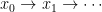
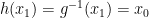
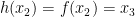
Theorem: If there is an injective map from a set to and also an injective map from to , then the sets and have the same cardinality.

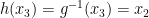
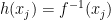
Recall that a map is injective provided implies that , surjective if its range is all of , and bijective if it is both injective and surjective. We can thank the great nonexistent French mathematician Nicolas Bourbaki for standardizing these terms, noting that sur is French for “on.” The definition of and having the same cardinality is that there exists a map that is bijective. All of this applies for sets of any cardinality, finite or infinite.

CBT and Graph Theory

The key insight for me is to think about CBT as a theorem about directed bipartite graphs. This insight is due to Gyula König. He was a set theorist, but his son became a famous graph theorist. So perhaps this explains the insight. The ideas which follow are related to proofs in a 1994 paper by John Conway and Peter Doyle, which is also summarized here and relates to this 2000 note by Berthold Schweizer. We mentioned Doyle recently here.

A directed bipartite graph has two sets of disjoint vertices the left side and the right side. All edges go only from a left vertex to a right or from a right to a left.

In a directed graph every vertex has an out-degree and an in-degree: the former is the number of edges leaving the vertex and the latter is number of edges that enter the vertex.

In order to study CBT via graph theory we need to restrict our attention to a special type of directed bipartite graph. Say is an injective bipartite graph provided it is a directed bipartite graph with the following restrictions:

1. The out-degree of all vertices is one;
2. The in-degree of all vertices is at most one.

The claim is:

Theorem 2 Any injective directed bipartite graph has the same number of left and right vertices.

This theorem proves CBT. Let be the injective maps from and as above, where we assume that and are disjoint. Then define as a directed bipartite graph with as the left vertices and as the right. There is an edge from to and an edge from to . The graph is injective: property (1) follows since both and are functions, and property (2) follows since both and are injective.

Basic Properties

From now on, let be an injective directed bipartite graph with left vertices and right vertices . Note that every path in must alternate left and right vertices, because is bipartite.

The key concept is that of a maximal path. A maximal path in is a path that cannot be extended on either end. One simple example of a maximal path is a cycle:

However, in an infinite graph there can be other maximal paths. One is a two-way infinite path

And the other is a one-way infinite path

Here there is no edge into . A simple but important observation is that two distinct maximal paths have no vertices in common.

A final basic observation is the following: Suppose that is partitioned into sets

and is also partitioned into

If for each index , there is a bijection from to , then and have the same cardinality. Let’s call this the partition trick.

I am trying to include even the simplest idea of the proof. Is this helpful, or am I being too detailed? You can skip the easy parts, but my experience is that people sometimes get hung up on the most basic steps of a proof. This is why I am including all the details.

Finite Graphs

Let’s prove the theorem for the case when the graph is finite.

Theorem 3 An injective directed finite bipartite graph has the same number of left and right vertices.

We had better be able to do this. We claim the following decomposition fact: The graph is the union of disjoint cycles. This follows since the only maximal paths in are cycles—this uses that is finite.

This proves the theorem, since each cycle has the same number of left vertices as right, and therefore each cycle has a bijection from left to right. By the partition trick the theorem is proved.

So far, pretty easy.

Infinite Graphs

We now will prove the theorem in the case that is infinite. By the partition trick we need only show that there is a bijection on each maximal path. This is clear for cycles—it is the same as above even for a two-way infinite cycle: since it alternates left and right, we can just take to be the map that defines the bijection. The case of a one-way infinite path is just barely harder. Let

be such a path. If 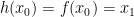is a left node, then we define and to make the bijection go back and forth over the first edge in the path, then and similarly for the third edge, and so on. If is a right vertex, we instead get for even and for odd . Pretty easy too.

Some Puzzles About The Proof

Even thought the proof is about any sets of any cardinality—as large as you like—the proof employs paths that are either finite or countable in length. This seems a bit strange—no? I have wondered whether this ability to work only with such paths can be exploited in some manner. I do not see how to use this fact. Oh well.

The countable case matters most in computability and complexity theory. John Myhill proved that if and are computable, then so is some bijection . This at first seems strange—how can you recognize you are in an infinite cycle?—but it works this way in finite stages : At any odd stage, let be the least number for which has not been defined. Let . If has not been listed as a value of at a previous stage, put . Else, we have already handled some such that . Then since we hadn’t handled , and since is injective. So put . If has not already been listed as a value of , then put . Else, we have already handled such that , and we repeat with …

Eventually we must exhaust the finitely many strings previously placed into the range of , and the first new string becomes . Since is a value of , inductively we are also preserving the property . Next, however, we need to do an even stage. Then we call the least number not already placed into the range of , and consider . Then . If is not already in the domain of , we define . Else, we have already handled some such that , and inductively , so we repeat with . Eventually we obtain not already in the domain of , and define . This entire process computably defines both and in “zipper” fashion for any or , yielding a computable bijection of that induces an isomorphism between and .

In complexity theory, we want to be polynomial-time computable if and are. This is true provided and are length increasing as well as polynomial-time invertible, but not by the same algorithm—given an we can’t go back and do all previous stages in polynomial time. Instead, the algorithm found by Leonard Berman and Juris Hartmanis alternates trying

as far as possible, which must stop within length-of- steps because the length is always decreasing. If fails first then , else .

This is the second puzzle: why do the ideas have to be so different? Is there a common formulation that might be used with other levels and kinds of complexity? The Berman-Hartmanis proof does resemble the one-way-infinite path case more than it does Myhill’s proof.

Open Problems

Does this help in understanding the proof? There are many proofs of CBT on the web, perhaps this is a better version. Take a look.

[fixed “domain”->”range” in one place in Myhill proof; worked around WordPress bug with length-of-x for |x|.]