Introduction

Early decentralized exchange (DEX) proposals took their inspiration from classical exchange markets and made use of order books to match sell and buy orders. Although these proposals achieved to be non-custodial exchanges, they turned out to be not very good in practice. The main reason for this is that an order book has a linear increase in storage and often even polynomial increase in computation with respect to the number of orders (see [1] , p. 2). This in turn — when implemented as smart contracts — caused far too high costs in fees making these solutions infeasible. Several approaches came up which run the order book offchain to reduce costs. This line of research continues to grow further using for example advanced cryptography (StarkDex) or exploiting batch ring trades (Gnosis).

A complementary approach to offchain order books for decentralized exchanges uses the concept of automated market makers (AMMs). The great advantage of such protocols are that they only require constant space and time interactions – unlike order books –, making non-custodial exchanges feasible.

In this post we look at the basics of the following three AMM projects: Uniswap, Balancer, and Curve. We shed some light on what they have in common, and try to understand in which aspects they are different from each other. The exposition takes a simplified view considering only trading markets with two tokens. This demonstrates already the essential points without getting lost in greater complexity. For those who want to understand the general case we provide links to further literature discussing the general case in even more depth.

The Formulas Behind Uniswap, Balancer, and Curve

In all three protocols there are two main agents involved. First, there are liquidity providers who deposit an amount of token t1 and a corresponding amount of token t2 to reserve pools R1 and R2. Secondly, there are traders who buy an amount Δ1 of token t1 for a specified amount Δ2 of token t2 (always assuming Δ1 ≤ R1). And, it is exactly the job of the automated market maker to define the price for t1 expressed in t2. This is achieved by the following very general pattern:

CORE PRINCIPAL: Suppose a trader wants to buy Δ1 tokens t1. We describe the market maker in terms of a trading function ψ (as in [1]). Such a trading function takes as input the actual reserve sizes R1, R2, as well as the trading amounts Δ1, Δ2, and maps these arguments to the value ψ(R1, R2,Δ1,Δ2). The terminology of constant function market maker (CFMM) stems from the constraint that the value of ψ has to be the same before and after the trade, i.e.

This constraint allows us to determine (in all our three cases uniquely) the amount Δ2 the trader has to pay for buying Δ1 tokens t1, and the smart contract accepts the trade only when the equation (1) holds true. After each trade the reserves become updated to R1 ← R1 – Δ1, and R2 ← R2 + Δ2.

PRICE IMPACT FUNCTION: Each trade of an amount of Δ1 tokens t1 has an impact on its price, since the reserve sizes are changing. In practice, if there is a significant difference between the price of the AMM and an external reference market, an arbitrage dealer will take this opportunity which balances the AMM price. The price impact of a trade of selling Δ1 tokens t1 is (mathematically speaking) the derivative of Δ2 considered as a function in Δ1, i.e.

We will exemplify this definition in the next section based on our three AMMs. With this definition at hand, the marginal price (infinitesimal small trade) of token t1 is just m := g(0).

Trading Functions and Marginal Prices

In this section we present the trading functions of Uniswap, Balancer and Curve, and their price impact functions. After passing through some mathematical formulas, we demonstrate in an example, how these different choices can be interpreted.

UNISWAP: The trading function of Uniswap is the product of the updated reserves

and the constraint (1) takes the form of

The price in t2 can be calculated by bringing all other terms of equation (2) to the right: Δ2 = (R1 * R2) / (R1 – Δ1) – R2. The price impact function of buying Δ1 tokens is then

As a special case, we get the marginal price mu = gu(0) = R2/R1 for Uniswap.

BALANCER: The trading function of Balancer is the weighted product of the updated reserves

where wi is in the interval (0, 1) and must satisfy w1 + w2 = 1. The constraint (1) then reads as

Similarly as above, the price in t2 can be calculated by bringing all remaining terms of equation (3) to the right-hand side:

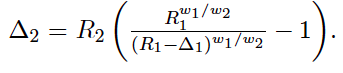
The price impact of buying of Δ1 tokens is then

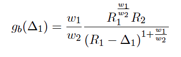
As a special case, we get the marginal price mb = gb(0) = w1/w2 * R2/R1.

Remark: The weights w1, w2 have an interpretation in terms of the total market value. Namely, when considering the two token market value in one or the other token, w1 reflects the share of token t1 and w2 reflects the share of token t2 (see [4]). When we choose w1 = w2 = 1/2, then we discover the Uniswap case as a specialization of Balancer.

CURVE: The trading function of Curve is a linear combination of the sum and the product of the updated reserves

with α, β ≥ 0. Again, but this time with some more effort, one can find (see [1])

where k = ψc(R1;R2; 0; 0). The price impact of buying Δ1 tokens is a bit more complicated to derive, but once done some work, one finds

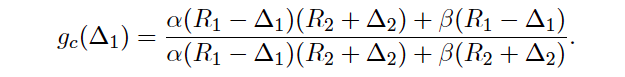
As a special case, we get the marginal price mc = gc(0) = (α + β (R12R2)-1)/ (α + β (R1R22)-1).

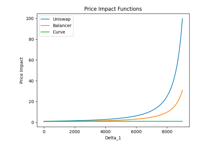
EXAMPLE. Each trade in a CFMM affects the price of the traded token, and the trade size even impacts the price in the same trade (“slippage”). This change in price depends heavily on the trading function of the market maker. Figure 1 shows the price impact functions we derived above for Uniswap, Balancer, and Curve. In this example we assume the reserves to be equal, namely R1= R2 = 10000. The marginal price of Uniswap is gu(0) = 1, for Balancer gb(0) = w1/w2, and for Curve the marginal price is gc(0) = 1. It becomes immediately visible that Curve’s AMM has for lower trade volumes more stable prices, making it attractive for traders between stable coins (where R1 = R2). Approaching the reserve size R1 Curve’s price impact function rapidly increases as well, but only when it is very close to the reserve size.

Figure 1: Price impact functions for Uniswap, Balancer, and Curve with reserves R1 = R2 = 10000, w1 = 0.6 and w2 = 0.4 for Balancer, and  α= 1 and β = 3 for Curve.

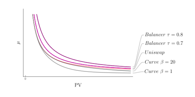
Another interesting quantity is the curvature μ of the price impact function, which is formally defined as g'(0) and satisfies g(Δ1) – g(0) ≤μg(0) (assuming g to be a convex function). It describes the change of the price with respect to the marginal price. Figure 2 shows how this bound on the price change varies with respect to the volume of the market, i.e the portfolio values PV of both token reserves.

Trading Functions with Fees

Usually fees are paid on the way in, i.e in the token t2, and the percentage fee of (1 – γ) charged Δ2 is paid out to the liquidity providers when they withdraw their funds (see next section for more details). Hence the trading function with fee of Uniswap, Balancer, and Curve from the previous section are slightly changed to

UNISWAP:

BALANCER:

CURVE:

Besides these changes, the reserves are updated in the same way as for the non-fee case, i.e. R1 ← R1 – Δ1, and R2 ← R2 + Δ2. The marginal price reflecting the trading fee are mu = 1/γ R2/R1 (Uniswap) and mb = 1/γ (w1R2)/(R1 w2) (Balancer). For Curve we will provide a corresponding formula in an update of this post.

Liquidity Provider Return and Other Topics

DEPOSIT and WITHDRAW: When a liquidity pool is created, its initial reserve balances are in 0, i.e. R1 = R2 = 0. The first liquidity provider sets the initial price of the pool by the amount of tokens t1 and t2 she decides to send to the pool. In case of Uniswap, she is incentivized to deposit an equal value of both tokens into the pool, otherwise an arbitrage dealer will use this opportunity. In the case of Balancer, also the weights w1,w2 can be set which incentivizes to deposit exactly this share of tokens to the pool. Subsequent liquidity providers must deposit pair tokens proportional to the current price (or make some corrections to it), otherwise they run the risk of being arbitraged as well.

LIQUIDITY PROVIDER RETURN: Whenever a liquidity provider deposits into a pool, she receives liquidity tokens in return. These tokens represent her contribution to the actual pool size. In order to withdraw, the liquidity provider must burn the liquidity tokens which gives her back the proportion of the reserve pool. Assuming a fixed market price, the liquidity provider will collect the same amount plus a return from fees which increased the pool size. (Some minor fees for withdrawing from reserves may apply!)

There is an empirical evidence that the shape of the price impact function and the liquidity provider’s return are correlated. As shown in Figure 1, Curve’s price impact function is flat around the “mean” (i.e. when R1 = R2 in the stable coin example) while the price impact function of Uniswap increases more rapidly. This invites stable coin traders to change higher amounts between stable coins in the Curve platform, which creates a higher trading volume. Therefore, a higher return is paid to liquidity providers in Curve, which, in fact, has the highest token volume locked (see here)! See [1], section 2, for a more general discussion. In the above scenario the market price of the tokens are supposed to be constant which can be assumed for stable coin pairs in Curve. For other coins, this is usually not the case, since slippage (see below) changes the token price. Until prices are not moved back to the “original” price, this may cause an impermanent loss. This loss becomes permanent when the liquidity provider withdraws before the price moves back. For more details see here.

NO-ARBITRAGE BOUND: Let’s look at the no-arbitrage bound. Again, (1- γ) is the percentage fee, and let mp the price of a reference market. When the marginal price of token t1 is smaller than the market price, i.e. m ≤ mp, there is a chance of a non-zero profit. With the same reasoning for the other way around, we have no-arbitrage opportunity state in Uniswap, when γ mp ≤ mu ≤ 1/γ mp, and for Balancer when γ mp ≤ mb ≤ 1/γ mp.

COST of MANIPULATION: If we denote by C(ε) the cost in t2 to change the market maker price mu of t1 to (1+ ε)mp, then [2], p.7, provides the following lower bound for Uniswap in the no-fee case:

An interesting observation is that the cost is bounded form below by the reserve size R2, i.e. the cost of manipulation becomes higher for markets with large liquidity pools. Similar formulas can derived for Balancer and Curve.

SLIPPAGE and FRONT-RUNNING: As we have seen in the example above, the current marginal prices can be changed by a large trade. This can be used to run an attack on a common trader — let’s name her Alice. By choosing a high gas fee, a malicious trader can achieve to put a buy order at price m1 just before the buy order of Alice who intended to buy with marginal price m1, but ends up buying at a higher price m2. The order of Alice goes through anyway, pushing the price up to a marginal price m3. Now the malicious trader sells at m3 making a profit. Since this attack puts a transaction before and after the transaction of Alice, it is also called a sandwich attack. See here for a good explanation and counter-measures.

References

[1] G. Angeris, A. Evans, T. Chitra; When does the tail wag the dog? Curvature and market making, 2020.

[2] G. Angeris et al.; An analysis of Uniswap markets, 2020.

[3] G. Angeris, T. Chitra; Improved Price Oracles: Constant Function Market Makers, 2020.

[4] F. Martinelli, N. Mushegian; Balancer white paper. 2019