Solving classic NP-hard problems such as 3-Coloring and Hamiltonian path with SAT solvers

In this blog we shall continue our discussion on a few NP-complete / NP-hard problems and will attempt to solve them (e.g., encoding the problem to satisfiability problem and solving with a SAT-solver) and the corresponding python implementations. The problems discussed here appeared as programming assignments in the coursera course Advanced Algorithms and Complexity. The problem statements are taken from the course itself.

Coloring a Graph with 3 colors using a SAT solver

Given a graph, we need to color its vertices into 3 different colors, so that any two vertices connected by an edge need to be of different colors. Graph coloring is an NP-complete problem, so we don’t currently know an efficient solution to it, and you need to reduce it to an instance of SAT problem which, although it is NP-complete, can often be solved efficiently in practice using special programs called SAT-solvers.

We can reduce the real-world problem about assigning frequencies to the transmitting towers of the cells in a GSM network to a problem of proper coloring a graph into 3 colors.Colors correspond to frequencies, vertices correspond to cells, and edges connect neighboring cells, as shown below.

Image taken from here

• We need to output a boolean formula in the conjunctive normal form (CNF) in a specific format. If it is possible to color the vertices of the input graph in 3 colors such that any two vertices connected by an edge are of different colors, the formula must be satisfiable. Otherwise, the formula must be unsatisfiable.
• We shall use pySAT SAT-solver to solve the clauses generated from the graph.
• In particular, if there are n nodes and m edges in the graph that is to be colored with 3 colors, we need to generate 3*n variables and 3*m + n clauses.
• The i-th vertex will correspond to 3 variables, with id i, n+i and 2*n+i. They will represent whether the node is to be colored by red, green or blue.
• Any two vertices forming an edge must not have the same color.
• Each vertex must be colored by one from the 3 colors.

The following python code snippet shows how the encoding needs to be implemented to output the desired clauses for the CNF, subsequently solved by the SAT-solver and the solution assignments is used to color the vertices of the graph. Again, there are following 3 basic steps:

• encode the input graph into SAT formula (reduce the 3-coloring problem to a satisfiability problem)
• solve with a SAT-solver and obtain the solution in terms of variable assignments
• Decode the solution — use the solution assignments by SAT-solver to color the vertices of the graph

import numpy as np
from pysat.solvers import Glucose3def get_colors(assignments):
    all_colors = np.array(['red', 'green', 'blue'])
    colors = {}
    for v in range(n):
	colors[v+1] = all_colors[[assignments[v]>0, \
	      assignments[n+v]>0, assignments[2*n+v]>0]][0]
	return colorsdef print_clauses(clauses):
    for c in clauses:
	vars = []
	for v in c:
    	   vars.append('{}x{}'.format('¬' if v < 0 else '', abs(v)))
	print('(' + ' OR '.join(vars) + ')')

def print_SAT_solution(assignments):
    sol = ''
    for x in assignments:
	sol += 'x{}={} '.format(abs(x),x>0)
    print(sol)

def solve_graph_coloring():
    # encode the input graph into SAT formula
    n_clauses = 3*m+n
    n_vars = 3*n
    clauses = []
    for u, v in edges:
 	clauses.append((-u, -v)) # corresponding to red color
	clauses.append((-(n+u), -(n+v))) # corresponding to green 
 	clauses.append((-(2*n+u), -(2*n+v))) # corresponds to blue
    for v in range(1, n+1):
        clauses.append((v, n+v, 2*n+v)) # at least one color
    print_clauses(clauses)
    # solve SAT and obtain solution in terms of variable assignments
    g = Glucose3()
    for c in clauses:
        g.add_clause(c)
    status = g.solve()
    assignments = g.get_model()
    print(status)
    print_SAT_solution(assignments)
    # use the solution assignment by SAT to color the graph
    colors = get_colors(assignments)
    print(colors)

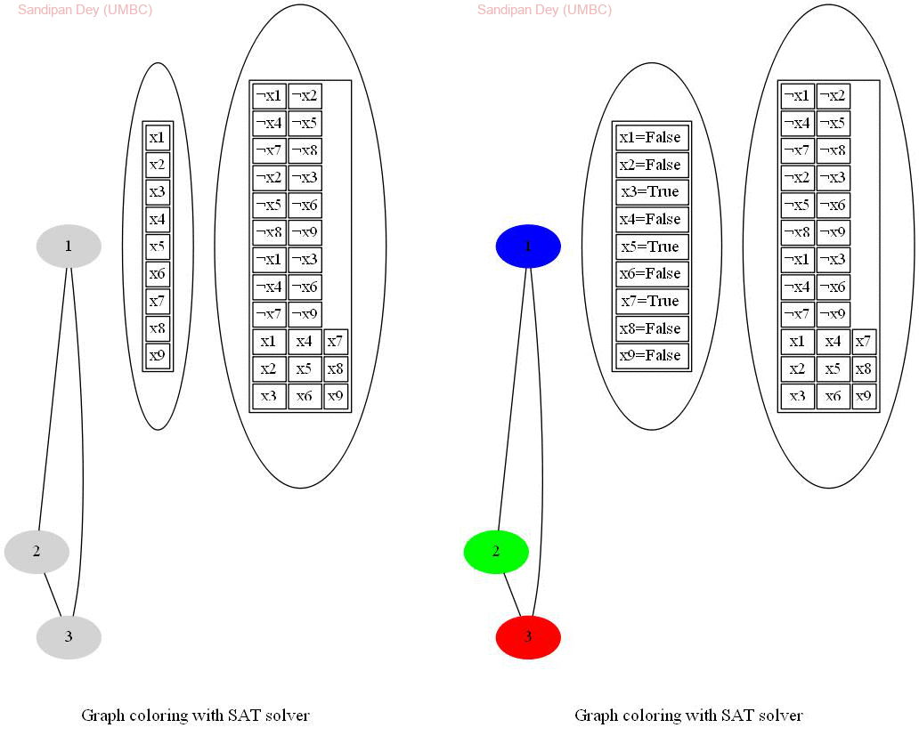
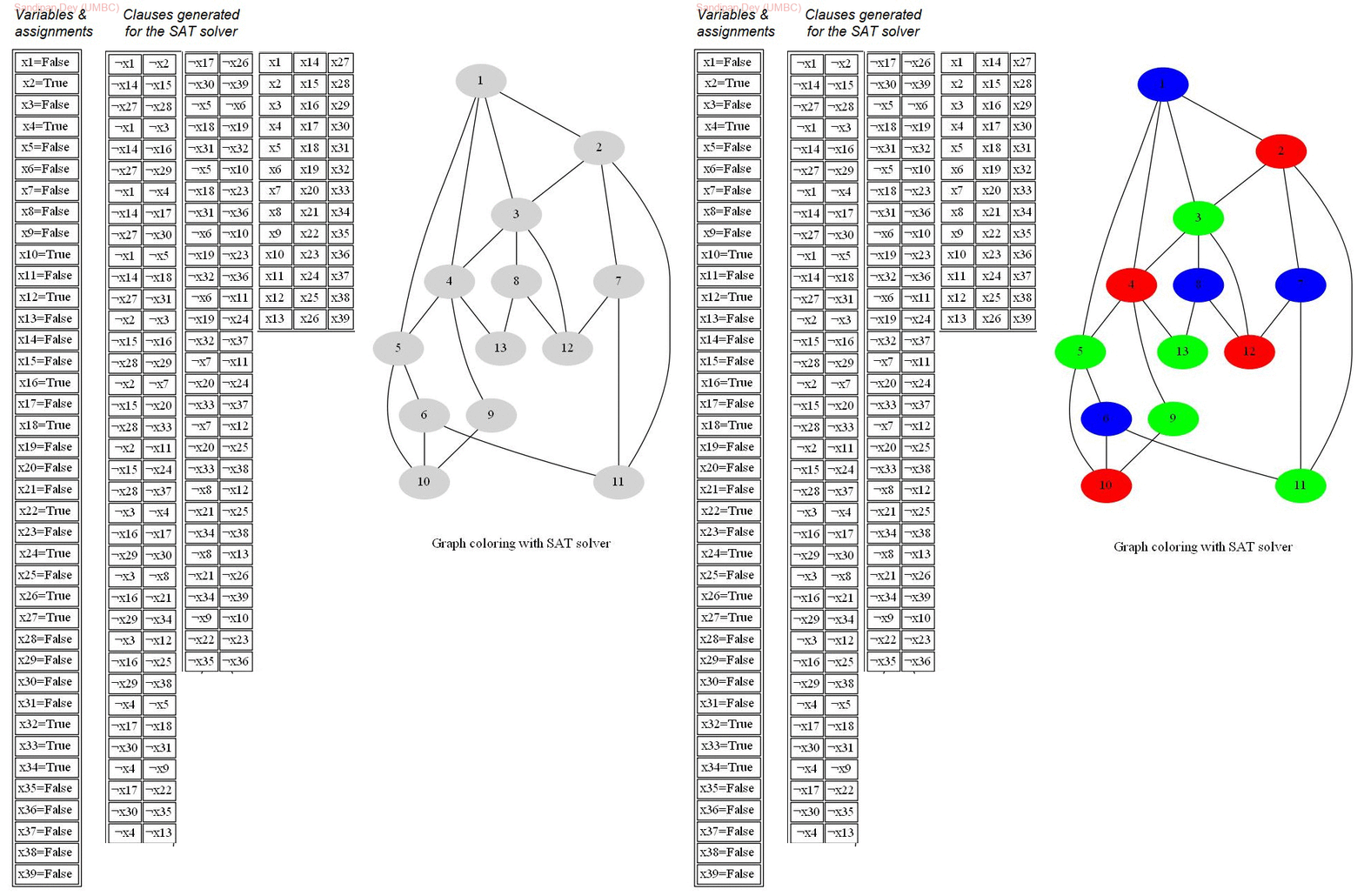
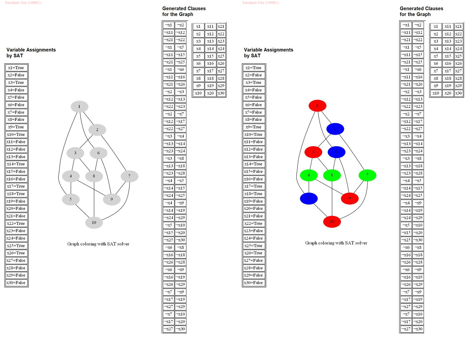
The following animations show the input graphs, the corresponding variables and clauses generated for the CNF to be solved with the SAT-solver, the solution obtained in terms of truth-assignments of the variables and then how they are used solve the graph-coloring problem, to color the graph with 3 colors. Each row in the right subgraph represents a clause in the CNF.

Image by AuthorImage by AuthorImage by Author

The last graph is the Petersen graph, that has chromatic number 3, so can be colored with 3 colors and a 3-coloring solution is obtained by the SAT-solver output assignments.

Now, the following example shows an input graph which is NOT 3-colorable, with the CNF formed by the clauses generated to be solved by the SAT-solver being unsatisfiable / inconsistent.

Image by Author

Solving the Hamiltonian Path problem with SAT-solver

In this problem, we shall learn how to solve the classic Hamiltonian Path problem, by designing and implementing an efficient algorithm to reduce it to SAT.

The following python snippet shows

1. how the Hamiltonian Path problem is reduced to SAT

2. Then it’s solved by the pysat SAT-solver.

3. The solution is interpreted to construct the Hamiltonian path for the following input graphs.

def get_hamiltonian_path(assignments):
    path = [None]*n
    for i in range(n):
	for j in range(n):
  	   if assignments[i*n+j] > 0: # True
		path[i] = j+1
    return path

def reduce_Hamiltonian_Path_to_SAT_and_solve(edges):

def index(i, j):
	return n*i + j + 1

m = len(edges)
    n_clauses = 2*n + (2*n*n-n-m)*(n-1)
    n_vars = n*n
    clauses = []

for j in range(n):
  	clause = []
	for i in range(n):
    	    clause.append(index(i,j))
	clauses.append(clause)
    for i in range(n):
	clause = []
	for j in range(n):
  	    clause.append(index(i,j)) 
	clauses.append(clause)
    for j in range(n):
 	for i in range(n):
   	    for k in range(i+1, n):
		clauses.append((-index(i,j), -index(k,j)))
    for i in range(n):
        for j in range(n):
   	    for k in range(j+1, n):
	        clauses.append((-index(i,j), -index(i,k)))
    for k in range(n-1):
        for i in range(n):
  	    for j in range(n):
		if i == j: continue
	  	    if not [i+1, j+1] in edges:
			clauses.append((-index(k,i), -index(k+1,j)))
    print_clauses(clauses)
    g = Glucose3()
    for c in clauses:
	g.add_clause(c)
    status = g.solve()
    assignments = g.get_model()
    print(status)
    print_SAT_solution(assignments)
    path = get_hamiltonian_path(assignments)
    print(path)

The following figure shows the output Hamiltonian Path obtained for the line input graph using the solution obtained by SAT-solver.

Image by Author

The following figure shows the Hamiltonian Path obtained with the SAT-solver for the input Petersen’s graph, which indeed has a Hamiltonian Path.

Image by Author

To be continued…