

Bezier Curves from the Ground Up
source link: http://jamie-wong.com/post/bezier-curves/
Go to the source link to view the article. You can view the picture content, updated content and better typesetting reading experience. If the link is broken, please click the button below to view the snapshot at that time.

Bezier Curves from the Ground Up
This post is also available in Japanese: 一から学ぶベジェ曲線.
How do you describe a straight line segment? We might think about a line segment in terms of its endpoints. Let’s call those endpoints P0 P_0 P0 and P1 P_1 P1.
P0 P1
To define the line segment rigorously, we might say “the set of all points along the line through P0 P_0 P0 and P1 P_1 P1 which lie between P0 P_0 P0 and P1 P_1 P1“, or perhaps this:
L(t)=(1−t)P0+tP1,0≤t≤1 L(t) = (1 - t) P_0 + t P_1, 0 \le t \le 1 L(t)=(1−t)P0+tP1,0≤t≤1
Conveniently, this definition let’s us easily find the coordinate of the point any portion of the way along that line segment. The midpoint, for instance, lies at L(0.5) L(0.5) L(0.5).
P0 P1 L(0.5)
We can, in fact, linearly interpolate to any value we want between the two points, with arbitrary precision. This allows us to do fancier things, like trace the line by having the t t t in L(t) L(t) L(t) be a function of time.
P0 P1L(0.40)
If you got this far, you might now be wondering, “What does this have to do with curves?“. Well, it seems quite intuitive that you can precisely describe a line segment with only two points. How might you go about precisely describing this?
It turns out that this particular kind of curve can be described by only 3 points!
P0 P1 P2
This is called a Quadratic Bezier Curve. A line segment, donning a fancier hat, might be called a Linear Bezier Curve. Let’s investigate why.
First, let’s consider what it looks like when we interpolate between P0 P_0 P0 and P1 P_1 P1 while simultaneously interpolating between P1 P_1 P1 and P2 P_2 P2.
P0 P1 P2 B0,1(0.40) B1,2(0.40)
Now let’s linearly interpolate between B0,1(t) B_{0, 1}(t) B0,1(t) and B1,2(t) B_{1, 2}(t) B1,2(t)…
P0 P1 P2 B0,1,2(0.40)
Notice that the equation for B0,1,2(t) B_{0, 1, 2}(t) B0,1,2(t) looks remarkably similar to the equations for B0,1 B_{0, 1} B0,1 and B1,2 B_{1, 2} B1,2. Let’s see what happens when we trace the path of B0,1,2(t) B_{0, 1, 2}(t) B0,1,2(t).
P0 P1 P2
We get our curve!
P0 P1 P2
Higher Order Bezier Curves
Just as we get a quadratic bezier by interpolating between two linear bezier curves, we get a cubic bezier curve by interpolating between two quadratic bezier curves:
P0 P1 P2 P3
P0 P1 P2 P3
You may have a sneaking suspicion at this point that there’s a nice recursive definition lurking here. And indeed there is:
Or, expressed (concisely but inefficiently) in TypeScript, it might look like this:
type Point = [number, number];
function B(P: Point[], t: number): Point {
    if (P.length === 1) return P[0];
    const left: Point = B(P.slice(0, P.length - 1), t);
    const right: Point = B(P.slice(1, P.length), t);
    return [(1 - t) * left[0] + t * right[0],
            (1 - t) * left[1] + t * right[1]];
}
// Evaluate a cubic spline at t=0.7
B([[0.0, 0.0], [0.0, 0.42], [0.58, 1.0], [1.0, 1.0]], 0.7)
Cubic Bezier Curves in Vector Images
As it happens, cubic bezier curves seem to be the right balance between simplicity and accuracy for many purposes. These are the kind of curves you’ll most often see in vector editing tools like Figma.
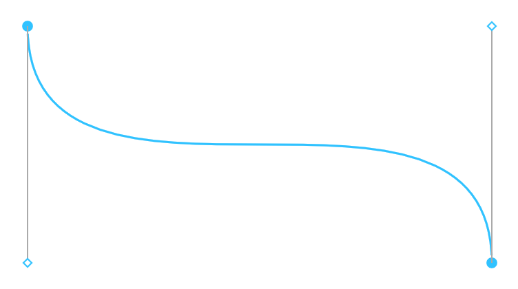
You can think of the two filled in circles ● as P0 P_0 P0 and P3 P_3 P3, and the two diamonds ◇ as P1 P_1 P1 and P2 P_2 P2. These are the fundamental building blocks of more complex curved vector constructions.
Font glyphs are specified in terms of bezier curves in TrueType (.ttf) fonts.
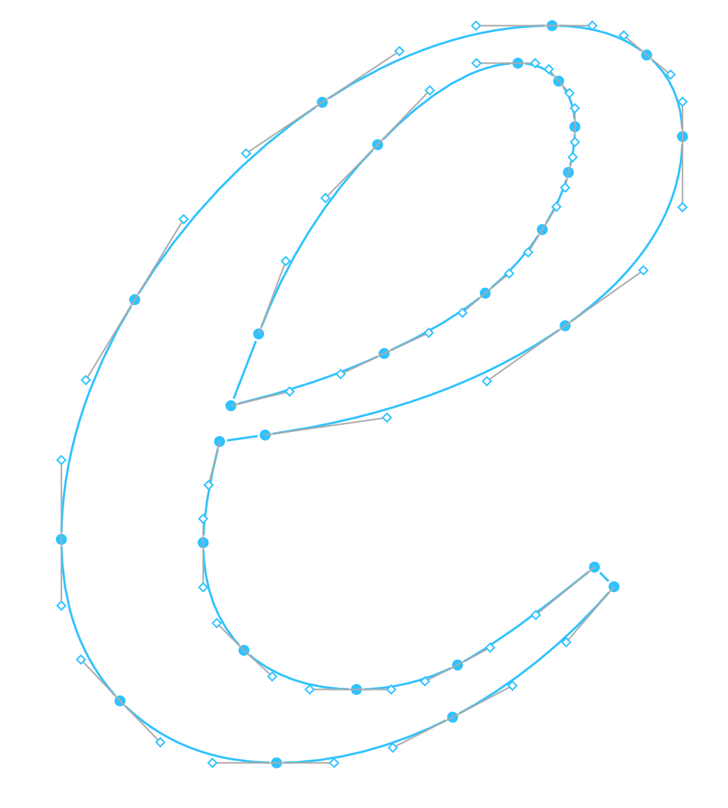
The Scalable Vector Graphics (.svg) file format uses bezier curves as one of its two curve primitives, which are used extensively in this:

Cubic Bezier Curves in Animation
While bezier curves have their most obvious uses in representing spacial curves, there’s no reason why they can’t be used to represented curved relationships between other quantities. For instance, rather than relating x x x and yy y, CSS transition timing functions relate a time ratio with an output value ratio.
Transition timing functions defined by bezier curves
Cubic bezier curves are one of two ways of expressing timing functions in CSS
(steps() being the other). The cubic-bezier(x1, y1, x2, y2) notation
for CSS timing functions specifies the coordinates of P1 P_1 P1 and P2 P_2
P2 of a cubic bezier curve.

transition-timing-function: cubic-bezier(x1, y1, x2, y2)Let’s pretend we’re trying to animate an orange ball moving. In all of these diagrams, the red lines representing time move at a constant speed.
linear (0.00, 0.00) (1.00, 1.00) ease (0.25, 0.10) (0.25, 1.00) ease-in (0.42, 0.00) (1.00, 1.00) ease-out (0.00, 0.00) (0.58, 1.00) ease-in-out (0.42, 0.00) (0.58, 1.00) (custom) (0.50, 1.00) (0.50, 0.00)
Why Bezier Curves?
Bezier curves are a beautiful abstraction for describing curves. The most commonly used form, cubic bezier curves, reduce the problem of describing and storing a curve down to storing 4 coordinates.
Beyond the efficiency benefits, the effect of moving the 4 control points on the curve shape is intuitive, making them suitable for direct manipulation editors.
Since 2 of the points specify the endpoints of the curve, composing many bezier curves into more complex structures with precision becomes easy. The exact specification of endpoints is always what makes it so convenient in the animation case: the only sensible value of the easing function at t=0% t = 0\% t=0% is the initial value, and the only sensible value at t=100% t = 100\% t=100% is the final value.
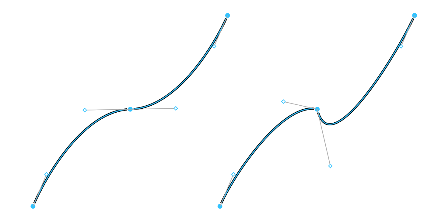
A less obvious benefit is that the line from P0 P_0 P0 to P1 P_1 P1 specifies the tangent of the curve leaving P0 P_0 P0. This means if you have two joint curves with mirrored control points, the slope at the join point is guaranteed to be the same on either side of the join.
A major benefit of mathematical construct like bezier curves is the ability to leverage decades of mathematical research to solve most problems you might run into, completely agnostic to the rest of your problem domain.
For instance, to make this post, I had to learn how to split a bezier curve at a given value of t t t in order to animate the curves above. I was quickly able to find a well written article on the matter: A Primer on Bézier Curves: Splitting Curves.
Resources and Further Reading
- A Primer on Bézier Curves in addition to having a description of using deCasteljau’s algorithm to draw and split curves, this free online book seems to be a pretty comprehensive intro.
- Bézier curve on Wikipedia shows many different mathematical formulas of bezier curves beyond the recursive definition shown here. It also contains the original animations that made bezier curves seem so evidently elegant to me.
Also a shoutout to Dudley Storey for his article Make SVG Responsive, which allowed all of the inline SVG in this article to work nicely on mobile.
Recommend
About Joyk
Aggregate valuable and interesting links.
Joyk means Joy of geeK