A simple weighted displacement difference test to evaluate place based crime int...

Table 1 explains the information needed to calculate the WDD. There are four areas; the treated area T, a control area comparable to the treated area Ct, a displacement area D, and a second control area comparable to the displacement area Cd. These are then indexed by counts of crime before the intervention took place with the subscript 0, and counts of crime in the post time period after the intervention took place with a subscript of 1. Note this is one more piece of additional information than the WDQ requires, a control area to correspond to the displacement area, which is sometimes considered in the evaluation literature but not frequently (Bowers et al. 2011a; Telep et al. 2014). We more critically discuss this unique requirement in a later section.

Based on this table, one can then identify the change in the treated, control, and displacement areas, subtracting the pre time period from the post time period.

The WDD is then calculated as:

For a simple example, say crime decreased in the treated area by 10 (from 30 to 20), decreased in the control-treatment area by 5 (from 30 to 25), increased in the displacement area by 2 (from 10 to 12), and increased in the control-displacement area by 1 (from 11 to 12). In this example, the WDD would equal − 10 − (− 5) + 2 − 1 = − 4. So although the treated area decreased by a larger margin, the control-treatment area also decreased (what might happen if crime is decreasing in the city overall). Because the displacement area also increased in crimes relative to the control-displacement area, the treatment effect is further reduced, but still has an estimate of decreasing 4 crimes in the combined treatment and displacement areas relative to their respective control trends.

Note in the case of spatial diffusion of benefits (Bowers et al. 2011b; Clarke and Weisburd 1994; Guerette and Bowers 2009), in which crime decreases were also observed in the displacement area relative to the control-displacement area, those additional crime reduction benefits would be added to the total crime reduction effects in the WDD. Thus the WDD is a not a direct analogy to the WDQ, but is more similar to the total net effects (TNE) estimate, which includes crime reductions (or increases) in both the treated and displacement areas in its calculation (Guerette 2009).Footnote 1

Given these are counts of crime, assuming these counts follow a Poisson distribution is not unreasonable. While no set of real data will exactly follow a theoretical distribution, several prior applications have shown this Poisson assumption to not be unreasonable in practice (Maltz 1996; Wheeler 2016). We later discuss how departures from this Poisson assumption, in particular how crime tends to be over-dispersed compared to the Poisson distribution (Berk and MacDonald 2008), will subsequently affect the proposed test statistic.

The Poisson distribution has the simplifying assumption that its mean equals its variance, and hence even with only one observed count, one can estimate the variance of the WDD statistic (Ractliffe 1964). Making the assumption that each of the observations are independent,Footnote 2 one then can calculate the variance of the WDD as below, where {\mathbb{V}}\left( X \right) is notation to be read as the variance of XFootnote 3:

Subsequently the test statistic to determine whether the observed WDD is likely due to chance given the null hypothesis that the WDD equals zero is then:

This test statistic, what we will refer to as Z_{\text{WDD}}, follows a standard normal distribution, e.g. ± 2 is a change that would only happen fewer than 5 times out of 100 tests if the null hypothesis of WDD equaling zero were true. One can then identify statistically significant decreases (or increases) in crime due to the intervention, while taking into account changes in the control areas as well as spatially displaced crime.

Note that the test statistic can still be applied even if one does not have a set of displacement and control-displacement areas. The user can simply set the displaced areas pre and post statistics to zero and conduct the test as is, since the zero counts do not add any extra variance into the statistic. This property can also be used to test the crime reduction effects in the treated and displaced areas independently (e.g. a crime reduction estimate in the treated area and a separate crime reduction estimate in the displaced area) if one so wishes.

The WDD test statistic is used, as opposed to the WDQ, as the ratios to calculate the quotient make the null distribution of the WDQ ill-defined, as the denominators can equal zero in some circumstances (Wheeler 2016). This property, especially for low crime counts, makes interpreting percentages very volatile (Wheeler and Kovandzic 2018). Examining the differences avoids this, but remains simple to understand and only requires slightly more work (identifying a matched control area for the displacement area) than the WDQ.

Table 2 illustrates an example of calculating the WDD using an example adapted from the appendix of Guerette (2009)—examining a strategy aimed at reducing crime in rental units in Lancashire, UK. Because this example did not have a control-displacement area, we add fictitious numbers for illustration purposes.

Based on Table 2, the individual differences over time are:

And subsequently the overall WDD for this example is then:

The variance of the WDD statistic then equals:

And so the Z_{\text{WDD}} test statistic then equals:

So in this case the reduction of a total of − 118 crimes results in a statistically significant reduction. A Z-statistic of − 2.98 has a two-tailed p value less than 0.003. The standard error of the test statistic (the square root of the variance), is approximately 40. One can use the same estimate of the standard error to estimate a confidence interval around the WDD statistic. In this case, a 95% confidence interval equals - 118 \pm 1.96 \cdot \sqrt {1568} \approx \left[ { - 196, - 40} \right].

Simulation of the null distribution of Z_{WDD}

To ensure the validity of the proposed test statistic, simulations of the null distribution were conducted to establish whether the test statistic follows a standard normal distribution (i.e. has mean of zero and a variance of one). This was accomplished by simulating random deviates from a Poisson distribution of a given mean, and calculating the changes in each of the treatment, control-treated, displacement, and control-displacement areas. For each simulation the different areas were given the same underlying Poisson mean both in the pre and post treatment period, so there are no actual changes from pre to post in any of the areas. Any inferences from the simulation that concluded the intervention decreased (or increased) crimes would therefore be false positives. This procedure establishes that the false positive rate for the Z_{\text{WDD}} statistic is near where it should be if it were distributed according to the standard normal distribution. Values were simulated from Poisson means of 5, 15, 25, 50, and 100.

Additionally, we conducted a simulation run in which the baseline Poisson mean was allowed to vary between the treated and displacement areas, but was again constrained to be equal in the pre and post time periods. For this simulation run, the Poisson means were randomly drawn from a uniform distribution ranging from 5 to 100, so either treated or displacement areas could have larger baseline counts of crime. The simulation was then conducted for 1,000,000 runs, where one run would provide a single estimate of the WDD and the Z_{\text{WDD}} test statistic.

Table 3 provides the test statistics for each of the extreme percentiles corresponding to the standard normal distribution. One can see that the WDD test statistic in the simulation near perfectly follows the standard normal distribution, and still provides a good fit even at the extreme quantiles. For example, one would expect a Z score of less than − 2.33 only 1% of the time according to the standard normal distribution with a mean of zero and a variance of one. In the simulation values this occurred at most 1.01% of the time (in the Poisson mean of 5), to a low of 0.98% of the time (with a Poisson mean of 15). One can read the other columns in a similar fashion and see that they are all quite close to the expected proportion of observations that should fall within each bin. Slight deviations are to be expected due to the stochastic nature of the simulation, but these statistics provide clear evidence that the null distribution of the test statistic does indeed follow a standard normal distribution. This is true both for the simulations in which the baseline mean number of crimes were constrained to be equal for both the treated and control areas, as well as the simulation run in which they were allowed to vary.Footnote 4

One may ask why not simply use the current WDQ or TNE and attempt to place standard errors around that estimate? Unfortunately, this is not possible because the variance of the WDQ and TNE cannot be analytically defined in the same manner as the WDD. Both the WDQ and the TNE will have differing distributions under the null of no change depending on the baseline counts of crime. Additionally the extreme quantiles of the null distribution of no change for each of those statistics are quite volatile, mainly because the denominators in either of the statistics (in multiple places) can have very small values, causing the entire statistic to result in extremely large values (if defined at all) in relatively regular situations.Footnote 5 This point is further illustrated in Additional file 1: Appendix, where we calculate the WDQ and TNE statistics for the same simulated values as the WDD and show their volatility when no changes are occurring in the underlying means for either treated, control, or displacement areas.

While this simulation is only of a limited set of values, and in reality the treated and displacement areas are unlikely to have the same baseline Poisson mean, this is inconsequential for the WDD statistic (as is shown for the last simulation condition where they are allowed to vary). As long as the underlying crime counts follow a Poisson distribution, Z_{\text{WDD}} will closely follow a standard normal distribution. It is not necessary to assume that all of the treated and displacement areas have the same underlying mean for this to be true for the WDD, nor is it necessary to have differing suggestions for the strength of evidence given different baseline crime counts. This is not the case though with the WDQ nor the TNE. One cannot give generalizable advice (such as, a TNE statistic of + 50 is strong evidence that the intervention was effective in reducing crimes) as it depends on the baseline crime counts as to whether a swing of that size would be expected by chance. The same issue affects the WDQ statistic. It is however possible to give general advice when calculating the WDD and its associated Z_{\text{WDD}} value.

A note on the power of the WDD test

Due to the volatility of crime statistics, one should be wary that even if there is some evidence of a crime reduction, this test will often fail to reject the null hypothesis of no change over time. This is because it is necessary to have an intervention with effects larger than the inherent changes one would expect with count crime data, and in the case of lower baseline counts this can be a difficult threshold to meet. As an example of this type of floor effect (McCleary and Musheno 1981) consider this example: say the intervention, control-treated, displacement, and displacement-treated area each have around 5 crimes on average. This would result in a standard error estimate of the test statistic of \sqrt {8 \cdot 5 } \approx 6.3. At a two-tailed alpha level of 0.05, one would need to have reduced over 12 crimes (two times the standard error) to reject the null that the WDD was equal to zero. This is a near-impossible standard to meet with a baseline of only 5 crimes in the treated area. In that case one would need some combination of eliminating nearly all of the crimes in the treated and displacement areas and/or increases of crimes in the control areas to actually conclude that a statistically significant crime reduction took place. In the case of low base rates of crime, it will be rare to find strong evidence of crime reductions using the WDD statistic.

Table 4 displays a set of recommendations, relating one-tailed p-values to general strength of evidence concerning a crime reduction. Z_{\text{WDD}} values under − 1.3 (a one-tailed p-value of 0.1) provide weak evidence of crime reduction benefits to the intervention, with stronger evidence as one obtains lower values of Z. Z values over − 1.3 but below zero are additionally evidence of crime reductions, but could occur frequently by chance even if the intervention had no effect on crime. Note that these are intended to be general guidelines to crime analysts and police practitioners, many of whom have little formal training in statistics. While one could argue about the labels or the thresholds used to assign different levels of evidence, the overall goal is to take into account that a small negative WDD can simply occur by chance, and so one needs to assess both the size of that reduction as well as the expected error.

Aggregating up more crimes makes the potential to identify a statistically significant crime reduction more realistic. Figure 1 displays a set of curves that show the necessary crime reductions needed given a particular average number of crimes within each of the treated, displacement, and matched control areas. For example, at an average of 100 crimes in each area, one needs to have a WDD of around 30 crimes to show weak evidence of effectiveness (those 30 crime reductions can count as a combination of the treatment area as well as diffusion of benefits in the displacement area). To obtain a one-tailed p-value of less than 0.05 it would take 40 or more crimes reduced. To reach the strong and very strong thresholds takes 57 and 76 crimes respectively. This is again a difficult standard even with a baseline of 100 crimes, as many interventions cannot be reasonably expected to reduce 100% of targeted crimes, and can only hope to reduce a sizable fraction in the best case scenario.

Fig. 1

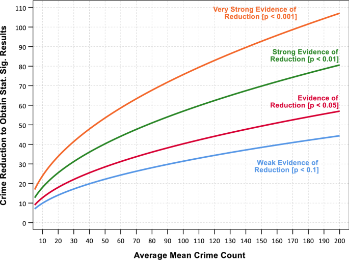
The standard error of the test statistic given average number of crimes per each period and within each area

Full size image

Because of this low power, one should keep in mind that failing to reject the null is not necessarily dispositive that the intervention was a failure. It could be the intervention is effective, it just does not prevent enough crimes to detect in the limited pre/post sample. Collecting more data over time, or expanding the intervention to additional areas, one might be able to identify reductions that appear to be larger than one would expect by chance.

Choosing reasonable control and displacement areas

One important distinction between the WDD and the WDQ is that the control areas for both the treated and the displacement areas should be comparable in terms of the linear differences in crime counts over time. As such, it is important for the control areas to have similar counts of crime to the treated and displacement areas, a requirement that is not as strict for the WDQ.

For a simple example of where a control area would not appear to be reasonable is if crime decreased in the treated area from 100 to 90, and crime decreased in the control area from 10 to 9. Ignoring the displacement areas, although each area decreased a comparable proportion of crimes, this would result in a WDD statistic of − 9.

A general way to understand this assumption is that if the treatment area decreased by n crimes (without any intervention), would it be reasonable for the control area to also decrease by n crimes? With the control area having so few crimes to begin with, this assumption (going from 10 to 0) seems unlikely. But if one were starting from a baseline of 60 crimes, going from 60 to 50 is more plausible.

This would suggest generally that reasonable control areas will have similar counts of crime compared to the treatment area. Preferably control areas would also be close to equal in geographic size as the treated area, although if the treatment is focused on a hot spot of crime for smaller jurisdictions that only have one hot spot this may not be feasible. But this is not an absolute requirement though—the control areas merely need to follow the same linear trends over time as the treatment area, which is likely to occur even if a control area is not a hot spot of crime. For example several long term evaluations of crime at micro places have shown that places with lower overall counts of crime tend to follow the same trajectory of crime decreases over time (Curman et al. 2015; Wheeler et al. 2016). In those cases, choosing several places in lower level trajectory groups to act as a control area for a high crime trajectory group location would be reasonable.

This also suggests displacement areas should have similar counts of crime compared to the treated/control areas if possible. While this is not necessary for the test statistic to behave appropriately as illustrated in the prior simulations, if one includes displacement areas that have substantially larger crime counts than the treated/control areas one will needlessly increase the variance of the test statistic, making it more difficult to detect if statistically significant crime reduction effects do occur. Typically one would assume displacement into only similar adjacent areas (Hesseling 1994), but if one wants to examine displacement into wider areas (Telep et al. 2014) it may make more sense to independently test the local and displacement effects, as opposed to pooling the areas into one test statistic.

With only counts of crime in the pre and post treatment periods, the linear change assumption cannot be verified; however, this assumption can be approximately verified (or refuted) if the analyst has access to more historical data before the treatment took place. For example, if crime in the treated area in the three years prior to the intervention grew from 80 to 90 to 100, and crimes in the control area grew from 40 to 50 to 60, this would be excellent evidence that the linear differences assumption is appropriate. Both series appear to be in-sync with one another, are subject to the same external forces that may influence overall crime trends, and that the linear changes appear to be in lockstep for each series. This behavior represents a realistic counterfactual condition that is often sought by evaluators, in that the control area is not only similar to the treatment area in a pre-intervention cross-sectional analysis, but also longitudinally. If the control area however grew from 15 to 30 to 60, the linear changes of 10 crimes appears to be inappropriate. They are both trending upwards, but not in equivalent magnitudes.

Similarly if the control area grew from 8 to 9 to 10, the series are both growing, but are parallel in their ratios, not on a linear scale. The linear assumption can also hold for control areas that have higher baseline counts of the crime than the treated area. A control area going from 150 to 160 to 170 would also be excellent evidence that the linear differences assumption is appropriate, even though it has a larger baseline count of crimes than the treated area.

Real world data are unlikely to be so convenient in verifying or refuting this assumption. Say if one had a control area that grew from 135 to 140 to 160, would the linear differences assumption be appropriate? While we cannot say for sure, one can keep in mind potential biases when choosing control areas. If you are choosing a control area that may change less than the treated area, in times of crime trending downward the intervention will likely appear more effective at reducing crime than it is in reality. If choosing a control area that may change less in times of crime trending upward the intervention will likely appear less effective than it is in reality. The obverse is true if choosing control areas that may change more than the treated and displacement areas when crime is trending downwards (will be more effective) or trending upwards (will be less effective). In times of no obvious trend of crime up or down, choosing control areas that have larger swings on average will introduce more variance in the statistic, but will not be consistently biased in either direction.

In the case that a single control area is reasonable as an overall measure of the expected crime change over time for both the treated and displacement areas, one can multiply the pre and post crime counts in the single control area by two and proceed with the statistic as usual. The WDD in that case would be {\Delta}T - 2 \cdot {\Delta}Ct + {\Delta}D. This might be reasonable if the treatment and displacement areas effectively cover an entire jurisdiction, have similar overall counts of crime, and control areas need to be drawn from a single neighboring jurisdiction. For all of these statistics, we recommend full and transparent disclosure of all the original counts (in addition to the differences over time) so that readers are able to appreciate any nuances in the data picture for all areas under examination, and factor this understanding into their interpretation of the study.