

Comprehensive Guide to Grouping and Aggregating with Pandas
source link: https://pbpython.com/groupby-agg.html
Go to the source link to view the article. You can view the picture content, updated content and better typesetting reading experience. If the link is broken, please click the button below to view the snapshot at that time.

Introduction
One of the most basic analysis functions is grouping and aggregating data. In some cases,
this level of analysis may be sufficient to answer business questions. In other instances,
this activity might be the first step in a more complex data science analysis. In pandas,
the
groupby
function can be combined with one or more aggregation
functions to quickly and easily summarize data. This concept is deceptively simple and most new
pandas users will understand this concept. However, they might be surprised at how useful complex
aggregation functions can be for supporting sophisticated analysis.
This article will quickly summarize the basic pandas aggregation functions and show examples of more complex custom aggregations. Whether you are a new or more experienced pandas user, I think you will learn a few things from this article.
Aggregating
In the context of this article, an aggregation function is one which takes multiple individual values and returns a summary. In the majority of the cases, this summary is a single value.
The most common aggregation functions are a simple average or summation of values. As of pandas 0.20, you may call an aggregation function on one or more columns of a DataFrame.
Here’s a quick example of calculating the total and average fare using the Titanic dataset (loaded from seaborn):
import pandas as pd
import seaborn as sns

df = sns.load_dataset('titanic')

df['fare'].agg(['sum', 'mean'])
sum     28693.949300
mean       32.204208
Name: fare, dtype: float64
This simple concept is a necessary building block for more complex analysis.
One area that needs to be discussed is that there are multiple ways to call an aggregation function. As shown above, you may pass a list of functions to apply to one or more columns of data.
What if you want to perform the analysis on only a subset of columns? There are two other options for aggregations: using a dictionary or a named aggregation.
Here is a comparison of the the three options:
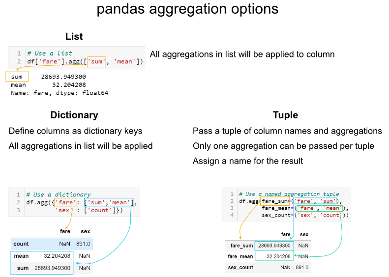
It is important to be aware of these options and know which one to use when.
The tuple approach is limited by only being able to apply one aggregation at a time to a
specific column. If I need to rename columns, then I will use the
rename
function
after the aggregations are complete. In some specific instances, the list approach is a useful
shortcut. I will reiterate though, that I think the dictionary approach provides the most
robust approach for the majority of situations.
Groupby
Now that we know how to use aggregations, we can combine this with
groupby
to summarize data.
Basic math
The most common built in aggregation functions are basic math functions including sum, mean, median, minimum, maximum, standard deviation, variance, mean absolute deviation and product.
We can apply all these functions to the
fare
while grouping by the
embark_town
:
agg_func_math = {
    'fare':
    ['sum', 'mean', 'median', 'min', 'max', 'std', 'var', 'mad', 'prod']
}
df.groupby(['embark_town']).agg(agg_func_math).round(2)

This is all relatively straightforward math.
As an aside, I have not found a good usage for the
prod
function which computes the
product of all the values in a group. For the sake of completeness, I am including it.
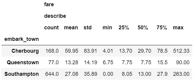
One other useful shortcut is to use
describe
to run multiple built-in aggregations
at one time:
agg_func_describe = {'fare': ['describe']}
df.groupby(['embark_town']).agg(agg_func_describe).round(2)
Counting
After basic math, counting is the next most common aggregation I perform on grouped data. In some ways, this can be a little more tricky than the basic math. Here are three examples of counting:
agg_func_count = {'embark_town': ['count', 'nunique', 'size']}
df.groupby(['deck']).agg(agg_func_count)
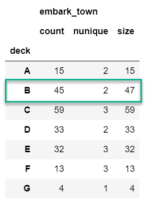
The major distinction to keep in mind is that
count
will not include
NaN
values whereas
size
will. Depending on the data set, this may or may not be a
useful distinction. In addition, the
nunique
function will exclude
NaN
values
in the unique counts. Keep reading for an example of how to include
NaN
in the
unique value counts.
First and last
In this example, we can select the highest and lowest fare by embarked town. One important
point to remember is that you must sort the data first if you want
first
and
last
to pick the max and min values.
agg_func_selection = {'fare': ['first', 'last']}
df.sort_values(by=['fare'],
            ascending=False).groupby(['embark_town'
                                        ]).agg(agg_func_selection)
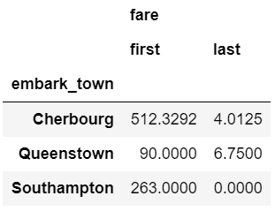
In the example above, I would recommend using
max
and
min
but I am including
first
and
last
for the sake of completeness. In other applications (such as
time series analysis) you may want to select the first and last values for further analysis.
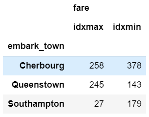
Another selection approach is to use
idxmax
and
idxmin
to select the index value
that corresponds to the maximum or minimum value.
agg_func_max_min = {'fare': ['idxmax', 'idxmin']}
df.groupby(['embark_town']).agg(agg_func_max_min)
We can check the results:
df.loc[[258, 378]]
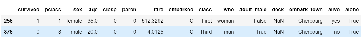
Here’s another shortcut trick you can use to see the rows with the max
fare
:
df.loc[df.groupby('class')['fare'].idxmax()]
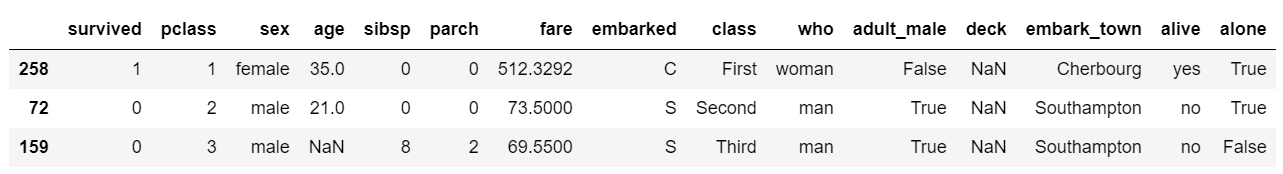
The above example is one of those places where the list-based aggregation is a useful shortcut.
Other libraries
You are not limited to the aggregation functions in pandas. For instance, you could use stats functions from scipy or numpy.
Here is an example of calculating the mode and skew of the fare data.
from scipy.stats import skew, mode
agg_func_stats = {'fare': [skew, mode, pd.Series.mode]}
df.groupby(['embark_town']).agg(agg_func_stats)
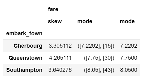
The mode results are interesting. The scipy.stats mode function returns
the most frequent value as well as the count of occurrences. If you just want the most
frequent value, use
pd.Series.mode.
The key point is that you can use any function you want as long as it knows how to interpret the array of pandas values and returns a single value.
Working with text
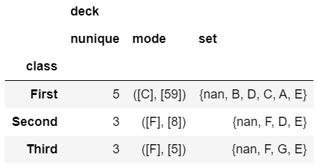
When working with text, the counting functions will work as expected. You can also use scipy’s mode function on text data.
One interesting application is that if you a have small number of distinct values, you can
use python’s
set
function to display the full list of unique values.
This summary of the
class
and
deck
shows how this approach can be useful for some data sets.
agg_func_text = {'deck': [ 'nunique', mode, set]}
df.groupby(['class']).agg(agg_func_text)
Custom functions
The pandas standard aggregation functions and pre-built functions from the python ecosystem will meet many of your analysis needs. However, you will likely want to create your own custom aggregation functions. There are four methods for creating your own functions.
To illustrate the differences, let’s calculate the 25th percentile of the data using four approaches:
First, we can use a partial function:
from functools import partial
# Use partial
q_25 = partial(pd.Series.quantile, q=0.25)
q_25.__name__ = '25%'
Next, we define our own function (which is a small wrapper around
quantile
):
# Define a function
def percentile_25(x):
    return x.quantile(.25)
We can define a lambda function and give it a name:
# Define a lambda function
lambda_25 = lambda x: x.quantile(.25)
lambda_25.__name__ = 'lambda_25%'
Or, define the lambda inline:
# Use a lambda function inline
agg_func = {
    'fare': [q_25, percentile_25, lambda_25, lambda x: x.quantile(.25)]
}

df.groupby(['embark_town']).agg(agg_func).round(2)
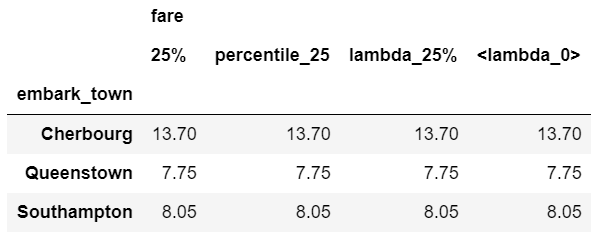
As you can see, the results are the same but the labels of the column are all a little different. This is an area of programmer preference but I encourage you to be familiar with the options since you will encounter most of these in online solutions.
Like many other areas of programming, this is an element of style and preference but I encourage you to pick one or two approaches and stick with them for consistency.
Custom function examples
As shown above, there are multiple approaches to developing custom aggregation functions. I will go through a few specific useful examples to highlight how they are frequently used.
In most cases, the functions are lightweight wrappers around built in pandas functions. Part of the reason you need to do this is that there is no way to pass arguments to aggregations. Some examples should clarify this point.
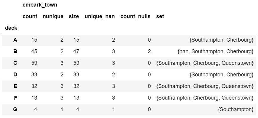
If you want to count the number of null values, you could use this function:
def count_nulls(s):
    return s.size - s.count()
If you want to include
NaN
values in your unique counts, you need to pass
dropna=False
to the
nunique
function.
def unique_nan(s):
    return s.nunique(dropna=False)
Here is a summary of all the values together:
agg_func_custom_count = {
    'embark_town': ['count', 'nunique', 'size', unique_nan, count_nulls, set]
}
df.groupby(['deck']).agg(agg_func_custom_count)
If you want to calculate the 90th percentile, use
quantile
:
def percentile_90(x):
    return x.quantile(.9)
If you want to calculate a trimmed mean where the lowest 10th percent is excluded, use the
scipy stats function
trim_mean
:
def trim_mean_10(x):
    return trim_mean(x, 0.1)
If you want the largest value, regardless of the sort order (see notes above about
first
and
last
:
def largest(x):
    return x.nlargest(1)
This is equivalent to
max
but I will show another example of
nlargest
below
to highlight the difference.
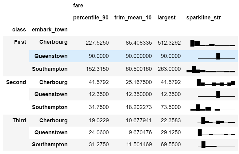
I wrote about sparklines before. Refer to that article for install instructions. Here’s how to incorporate them into an aggregate function for a unique view of the data:
def sparkline_str(x):
    bins=np.histogram(x)[0]
    sl = ''.join(sparklines(bins))
    return sl
Here they are all put together:
agg_func_largest = {
    'fare': [percentile_90, trim_mean_10, largest, sparkline_str]
}
df.groupby(['class', 'embark_town']).agg(agg_func_largest)
The
nlargest
and
nsmallest
functions can be useful for summarizing the data
in various scenarios. Here is code to show the total fares for the top 10 and bottom 10 individuals:
def top_10_sum(x):
    return x.nlargest(10).sum()

def bottom_10_sum(x):
    return x.nsmallest(10).sum()


agg_func_top_bottom_sum = {
    'fare': [top_10_sum, bottom_10_sum]
}
df.groupby('class').agg(agg_func_top_bottom_sum)
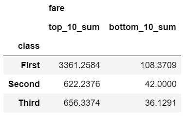
Using this approach can be useful when applying the Pareto principle to your own data.
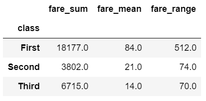
Custom functions with multiple columns
If you have a scenario where you want to run multiple aggregations across columns, then
you may want to use the
groupby
combined with
apply
as described in
this stack overflow answer.
Using this method, you will have access to all of the columns of the data and can choose the appropriate aggregation approach to build up your resulting DataFrame (including the column labels):
def summary(x):
    result = {
        'fare_sum': x['fare'].sum(),
        'fare_mean': x['fare'].mean(),
        'fare_range': x['fare'].max() - x['fare'].min()
    }
    return pd.Series(result).round(0)

df.groupby(['class']).apply(summary)
Using
apply
with
groupy
gives maximum flexibility over all aspects of
the results. However, there is a downside. The
apply
function is slow so this approach
should be used sparingly.
Working with group objects
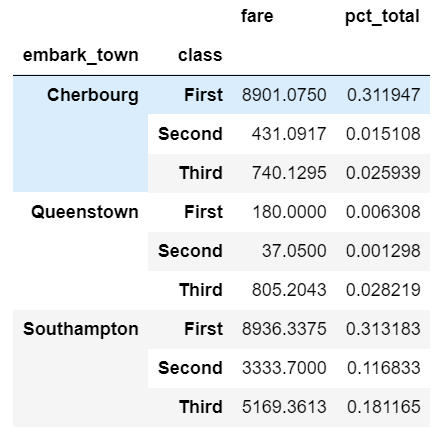
Once you group and aggregate the data, you can do additional calculations on the grouped objects.
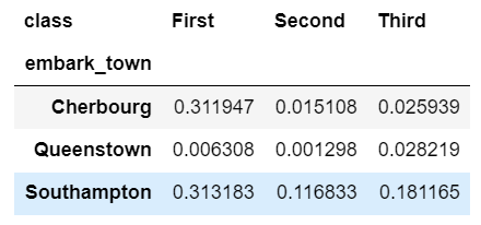
For the first example, we can figure out what percentage of the total fares sold
can be attributed to each
embark_town
and
class
combination. We use
assign
and a
lambda
function to add a
pct_total
column:
df.groupby(['embark_town', 'class']).agg({
    'fare': 'sum'
}).assign(pct_total=lambda x: x / x.sum())
One important thing to keep in mind is that you can actually do this more simply using a
pd.crosstab
as described in my previous article:
pd.crosstab(df['embark_town'],
            df['class'],
            values=df['fare'],
            aggfunc='sum',
            normalize=True)
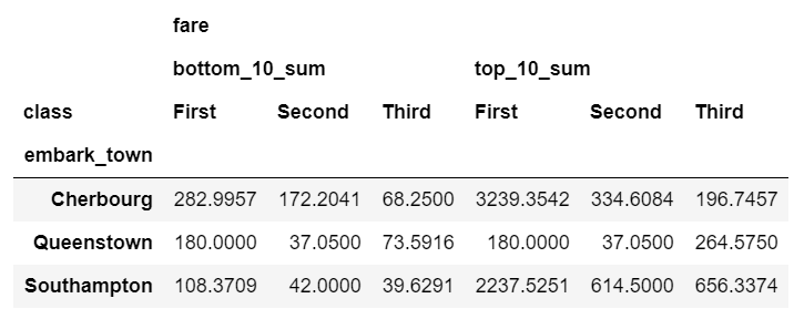
While we are talking about
crosstab
, a useful concept to keep in mind is that agg
functions can be combined with pivot tables too.
Here’s a quick example:
pd.pivot_table(data=df,
            index=['embark_town'],
            columns=['class'],
            aggfunc=agg_func_top_bottom_sum)
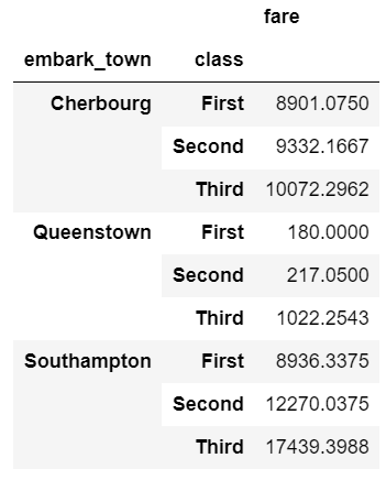
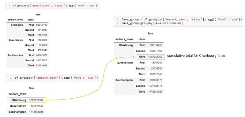
Sometimes you will need to do multiple groupby’s to answer your question. For instance, if we wanted to see a cumulative total of the fares, we can group and aggregate by town and class then group the resulting object and calculate a cumulative sum:
fare_group = df.groupby(['embark_town', 'class']).agg({'fare': 'sum'})
fare_group.groupby(level=0).cumsum()
This may be a little tricky to understand. Here’s a summary of what we are doing:
Here’s another example where we want to summarize daily sales data and convert it to a
cumulative daily and quarterly view. Refer to the Grouper article if you are not familiar with
using
pd.Grouper()
:
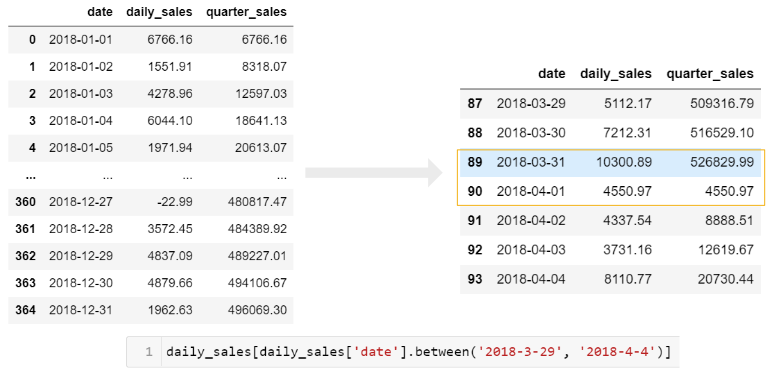
In the first example, we want to include a total daily sales as well as cumulative quarter amount:
sales = pd.read_excel('https://github.com/chris1610/pbpython/blob/master/data/2018_Sales_Total_v2.xlsx?raw=True')

daily_sales = sales.groupby([pd.Grouper(key='date', freq='D')
                            ]).agg(daily_sales=('ext price',
                                                'sum')).reset_index()
daily_sales['quarter_sales'] = daily_sales.groupby(
    pd.Grouper(key='date', freq='Q')).agg({'daily_sales': 'cumsum'})
To understand this, you need to look at the quarter boundary (end of March through start of April) to get a good sense of what is going on.
If you want to just get a cumulative quarterly total, you can chain multiple groupby functions.
First, group the daily results, then group those results by quarter and use a cumulative sum:
sales.groupby([pd.Grouper(key='date', freq='D')
            ]).agg(daily_sales=('ext price', 'sum')).groupby(
                pd.Grouper(freq='Q')).agg({
                    'daily_sales': 'cumsum'
                }).rename(columns={'daily_sales': 'quarterly_sales'})
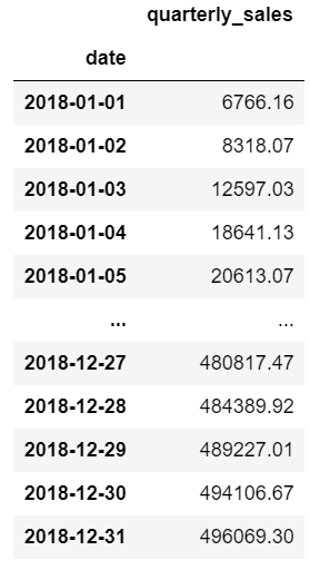
In this example, I included the named aggregation approach to rename the variable to clarify that it is now daily sales. I then group again and use the cumulative sum to get a running sum for the quarter. Finally, I rename the column to quarterly sales.
Admittedly this is a bit tricky to understand. However, if you take it step by step and build out the function and inspect the results at each step, you will start to get the hang of it. Don’t be discouraged!
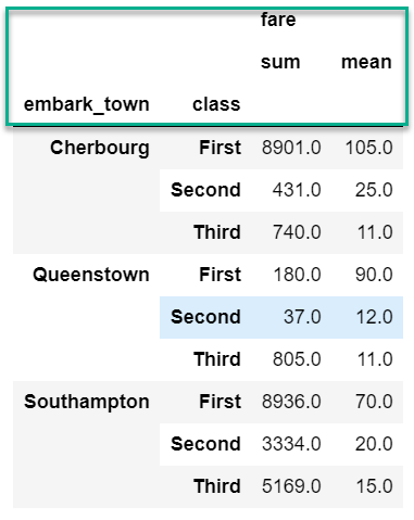
Flattening Hierarchical Column Indices
By default, pandas creates a hierarchical column index on the summary DataFrame. Here is what I am referring to:
df.groupby(['embark_town', 'class']).agg({'fare': ['sum', 'mean']}).round(0)
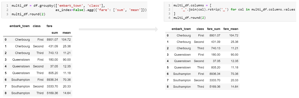
At some point in the analysis process you will likely want to “flatten” the columns so that there is a single row of names.
I have found that the following approach works best for me. I use the parameter
as_index=False
when grouping, then build a new collapsed column name.
Here is the code:
multi_df = df.groupby(['embark_town', 'class'],
                    as_index=False).agg({'fare': ['sum', 'mean']})

multi_df.columns = [
'_'.join(col).rstrip('_') for col in multi_df.columns.values
]
Here is a picture showing what the flattened frame looks like:
I prefer to use
_
as my separator but you could use other values. Just keep in mind
that it will be easier for your subsequent analysis if the resulting column names
do not have spaces.
Subtotals
One process that is not straightforward with grouping and aggregating in pandas is adding
a subtotal. If you want to add subtotals, I recommend the sidetable package. Here is how
you can summarize
fares
by
class
,
embark_town
and
sex
with a subtotal at each level as well as a grand total at the bottom:
import sidetable
df.groupby(['class', 'embark_town', 'sex']).agg({'fare': 'sum'}).stb.subtotal()
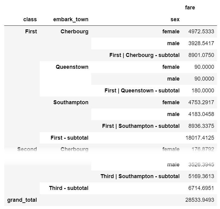
sidetable also allows customization of the subtotal levels and resulting labels. Refer to the package documentation for more examples of how sidetable can summarize your data.
Summary
Thanks for reading this article. There is a lot of detail here but that is due to how many different uses there are for grouping and aggregating data with pandas. My hope is that this post becomes a useful resource that you can bookmark and come back to when you get stuck with a challenging problem of your own.
If you have other common techniques you use frequently please let me know in the comments. If I get some broadly useful ones, I will include in this post or as an updated article.
image credit: Herman Traub
Recommend
About Joyk
Aggregate valuable and interesting links.
Joyk means Joy of geeK