

使用Transformer 模型进行时间序列预测的Pytorch代码示例
source link: https://www.51cto.com/article/780640.html
Go to the source link to view the article. You can view the picture content, updated content and better typesetting reading experience. If the link is broken, please click the button below to view the snapshot at that time.

使用Transformer 模型进行时间序列预测的Pytorch代码示例
时间序列预测是一个经久不衰的主题,受自然语言处理领域的成功启发,transformer模型也在时间序列预测有了很大的发展。本文可以作为学习使用Transformer 模型的时间序列预测的一个起点。
时间序列预测是一个经久不衰的主题,受自然语言处理领域的成功启发,transformer模型也在时间序列预测有了很大的发展。本文可以作为学习使用Transformer 模型的时间序列预测的一个起点。
数据集 这里我们直接使用kaggle中的 Store Sales — Time Series Forecasting作为数据。这个比赛需要预测54家商店中各种产品系列未来16天的销售情况,总共创建1782个时间序列。数据从2013年1月1日至2017年8月15日,目标是预测接下来16天的销售情况。虽然为了简洁起见,我们做了简化处理,作为模型的输入包含20列中的3,029,400条数据,。每行的关键列为' store_nbr '、' family '和' date '。数据分为三类变量:
1、截止到最后一次训练数据日期(2017年8月15日)之前已知的与时间相关的变量。这些变量包括数字变量,如“销售额”,表示某一产品系列在某家商店的销售额;“transactions”,一家商店的交易总数;' store_sales ',该商店的总销售额;' family_sales '表示该产品系列的总销售额。
2、训练截止日期(2017年8月31日)之前已知,包括“onpromotion”(产品系列中促销产品的数量)和“dcoilwtico”等变量。这些数字列由' holiday '列补充,它表示假日或事件的存在,并被分类编码为整数。此外,' time_idx '、' week_day '、' month_day '、' month '和' year '列提供时间上下文,也编码为整数。虽然我们的模型是只有编码器的,但已经添加了16天移动值“onpromotion”和“dcoilwtico”,以便在没有解码器的情况下包含未来的信息。
3、静态协变量随着时间的推移保持不变,包括诸如“store_nbr”、“family”等标识符,以及“city”、“state”、“type”和“cluster”等分类变量(详细说明了商店的特征),所有这些变量都是整数编码的。
我们最后生成的df名为' data_all ',结构如下:
categorical_covariates = ['time_idx','week_day','month_day','month','year','holiday']

 categorical_covariates_num_embeddings = []
 for col in categorical_covariates:
     data_all[col] = data_all[col].astype('category').cat.codes
     categorical_covariates_num_embeddings.append(data_all[col].nunique())

 categorical_static = ['store_nbr','city','state','type','cluster','family_int']

 categorical_static_num_embeddings = []
 for col in categorical_static:
     data_all[col] = data_all[col].astype('category').cat.codes
     categorical_static_num_embeddings.append(data_all[col].nunique())

 numeric_covariates = ['sales','dcoilwtico','dcoilwtico_future','onpromotion','onpromotion_future','store_sales','transactions','family_sales']

 target_idx = np.where(np.array(numeric_covariates)=='sales')[0][0]
在将数据转换为适合我的PyTorch模型的张量之前,需要将其分为训练集和验证集。窗口大小是一个重要的超参数,表示每个训练样本的序列长度。此外,' num_val '表示使用的验证折数,在此上下文中设置为2。将2013年1月1日至2017年6月28日的观测数据指定为训练数据集,以2017年6月29日至2017年7月14日和2017年7月15日至2017年7月30日作为验证区间。
同时还进行了数据的缩放,完整代码如下:
 def dataframe_to_tensor(series,numeric_covariates,categorical_covariates,categorical_static,target_idx):

     numeric_cov_arr = np.array(series[numeric_covariates].values.tolist())
     category_cov_arr = np.array(series[categorical_covariates].values.tolist())
     static_cov_arr = np.array(series[categorical_static].values.tolist())

     x_numeric = torch.tensor(numeric_cov_arr,dtype=torch.float32).transpose(2,1)
     x_numeric = torch.log(x_numeric+1e-5)
     x_category = torch.tensor(category_cov_arr,dtype=torch.long).transpose(2,1)
     x_static = torch.tensor(static_cov_arr,dtype=torch.long)
     y = torch.tensor(numeric_cov_arr[:,target_idx,:],dtype=torch.float32)

     return x_numeric, x_category, x_static, y


 window_size = 16
 forecast_length = 16
 num_val = 2

 val_max_date = '2017-08-15'
 train_max_date = str((pd.to_datetime(val_max_date) - pd.Timedelta(days=window_size*num_val+forecast_length)).date())

 train_final = data_all[data_all['date']<=train_max_date]
 val_final = data_all[(data_all['date']>train_max_date)&(data_all['date']<=val_max_date)]

 train_series = train_final.groupby(categorical_static+['family']).agg(list).reset_index()
 val_series = val_final.groupby(categorical_static+['family']).agg(list).reset_index()

 x_numeric_train_tensor, x_category_train_tensor, x_static_train_tensor, y_train_tensor = dataframe_to_tensor(train_series,numeric_covariates,categorical_covariates,categorical_static,target_idx)

 x_numeric_val_tensor, x_category_val_tensor, x_static_val_tensor, y_val_tensor = dataframe_to_tensor(val_series,numeric_covariates,categorical_covariates,categorical_static,target_idx)
数据加载器 在数据加载时,需要将每个时间序列从窗口范围内的随机索引开始划分为时间块,以确保模型暴露于不同的序列段。
为了减少偏差还引入了一个额外的超参数设置,它不是随机打乱数据,而是根据块的开始时间对数据集进行排序。然后数据被分成五部分——反映了我们五年的数据集——每一部分都是内部打乱的,这样最后一批数据将包括去年的观察结果,但还是随机的。模型的最终梯度更新受到最近一年的影响,理论上可以改善最近时期的预测。
 def divide_shuffle(df,div_num):
     space = df.shape[0]//div_num
     division = np.arange(0,df.shape[0],space)
     return pd.concat([df.iloc[division[i]:division[i]+space,:].sample(frac=1) for i in range(len(division))])

 def create_time_blocks(time_length,window_size):
     start_idx = np.random.randint(0,window_size-1)
     end_idx = time_length-window_size-16-1
     time_indices = np.arange(start_idx,end_idx+1,window_size)[:-1]
     time_indices = np.append(time_indices,end_idx)
     return time_indices

 def data_loader(x_numeric_tensor, x_category_tensor, x_static_tensor, y_tensor, batch_size, time_shuffle):

     num_series = x_numeric_tensor.shape[0]
     time_length = x_numeric_tensor.shape[1]
     index_pd = pd.DataFrame({'serie_idx':range(num_series)})
     index_pd['time_idx'] = [create_time_blocks(time_length,window_size) for n in range(index_pd.shape[0])]
     if time_shuffle:
         index_pd = index_pd.explode('time_idx')
         index_pd = index_pd.sample(frac=1)
     else:
         index_pd = index_pd.explode('time_idx').sort_values('time_idx')
         index_pd = divide_shuffle(index_pd,5)
     indices = np.array(index_pd).astype(int)

     for batch_idx in np.arange(0,indices.shape[0],batch_size):

         cur_indices = indices[batch_idx:batch_idx+batch_size,:]

         x_numeric = torch.stack([x_numeric_tensor[n[0],n[1]:n[1]+window_size,:] for n in cur_indices])
         x_category = torch.stack([x_category_tensor[n[0],n[1]:n[1]+window_size,:] for n in cur_indices])
         x_static = torch.stack([x_static_tensor[n[0],:] for n in cur_indices])
         y = torch.stack([y_tensor[n[0],n[1]+window_size:n[1]+window_size+forecast_length] for n in cur_indices])

         yield x_numeric.to(device), x_category.to(device), x_static.to(device), y.to(device)

 def val_loader(x_numeric_tensor, x_category_tensor, x_static_tensor, y_tensor, batch_size, num_val):

     num_time_series = x_numeric_tensor.shape[0]

     for i in range(num_val):

       for batch_idx in np.arange(0,num_time_series,batch_size):

           x_numeric = x_numeric_tensor[batch_idx:batch_idx+batch_size,window_size*i:window_size*(i+1),:]
           x_category = x_category_tensor[batch_idx:batch_idx+batch_size,window_size*i:window_size*(i+1),:]
           x_static = x_static_tensor[batch_idx:batch_idx+batch_size]
           y_val = y_tensor[batch_idx:batch_idx+batch_size,window_size*(i+1):window_size*(i+1)+forecast_length]

           yield x_numeric.to(device), x_category.to(device), x_static.to(device), y_val.to(device)
我们这里通过Pytorch来简单的实现《Attention is All You Need》(2017)²中描述的Transformer架构。因为是时间序列预测,所以注意力机制中不需要因果关系,也就是没有对注意块应用进行遮蔽。
从输入开始:分类特征通过嵌入层传递,以密集的形式表示它们,然后送到Transformer块。多层感知器(MLP)接受最终编码输入来产生预测。嵌入维数、每个Transformer块中的注意头数和dropout概率是模型的主要超参数。堆叠多个Transformer块由' num_blocks '超参数控制。
下面是单个Transformer块的实现和整体预测模型:
 class transformer_block(nn.Module):

     def __init__(self,embed_size,num_heads):
         super(transformer_block, self).__init__()

         self.attention = nn.MultiheadAttention(embed_size, num_heads, batch_first=True)
         self.fc = nn.Sequential(nn.Linear(embed_size, 4 * embed_size),
                                  nn.LeakyReLU(),
                                  nn.Linear(4 * embed_size, embed_size))
         self.dropout = nn.Dropout(drop_prob)
         self.ln1 = nn.LayerNorm(embed_size, eps=1e-6)
         self.ln2 = nn.LayerNorm(embed_size, eps=1e-6)

     def forward(self, x):

         attn_out, _ = self.attention(x, x, x, need_weights=False)
         x = x + self.dropout(attn_out)
         x = self.ln1(x)

         fc_out = self.fc(x)
         x = x + self.dropout(fc_out)
         x = self.ln2(x)

         return x

 class transformer_forecaster(nn.Module):

     def __init__(self,embed_size,num_heads,num_blocks):
         super(transformer_forecaster, self).__init__()

         num_len = len(numeric_covariates)
         self.embedding_cov = nn.ModuleList([nn.Embedding(n,embed_size-num_len) for n in categorical_covariates_num_embeddings])
         self.embedding_static = nn.ModuleList([nn.Embedding(n,embed_size-num_len) for n in categorical_static_num_embeddings])

         self.blocks = nn.ModuleList([transformer_block(embed_size,num_heads) for n in range(num_blocks)])

         self.forecast_head = nn.Sequential(nn.Linear(embed_size, embed_size*2),
                                            nn.LeakyReLU(),
                                            nn.Dropout(drop_prob),
                                            nn.Linear(embed_size*2, embed_size*4),
                                            nn.LeakyReLU(),
                                            nn.Linear(embed_size*4, forecast_length),
                                            nn.ReLU())

     def forward(self, x_numeric, x_category, x_static):

         tmp_list = []
         for i,embed_layer in enumerate(self.embedding_static):
             tmp_list.append(embed_layer(x_static[:,i]))
         categroical_static_embeddings = torch.stack(tmp_list).mean(dim=0).unsqueeze(1)

         tmp_list = []
         for i,embed_layer in enumerate(self.embedding_cov):
             tmp_list.append(embed_layer(x_category[:,:,i]))
         categroical_covariates_embeddings = torch.stack(tmp_list).mean(dim=0)
         T = categroical_covariates_embeddings.shape[1]

         embed_out = (categroical_covariates_embeddings + categroical_static_embeddings.repeat(1,T,1))/2
         x = torch.concat((x_numeric,embed_out),dim=-1)

         for block in self.blocks:
             x = block(x)

         x = x.mean(dim=1)
         x = self.forecast_head(x)

         return x
我们修改后的transformer架构如下图所示:
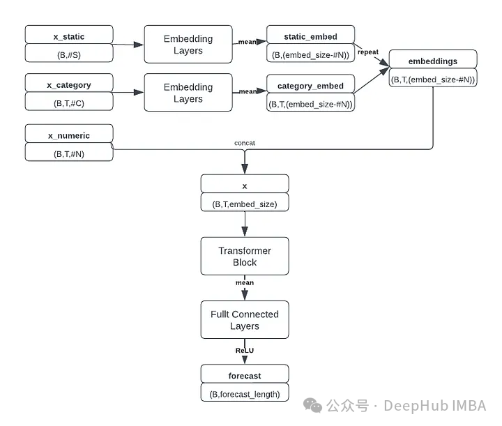
模型接受三个独立的输入张量:数值特征、分类特征和静态特征。对分类和静态特征嵌入进行平均,并与数字特征组合形成具有形状(batch_size, window_size, embedding_size)的张量,为Transformer块做好准备。这个复合张量还包含嵌入的时间变量,提供必要的位置信息。
Transformer块提取顺序信息,然后将结果张量沿着时间维度聚合,将其传递到MLP中以生成最终预测(batch_size, forecast_length)。这个比赛采用均方根对数误差(RMSLE)作为评价指标,公式为:

鉴于预测经过对数转换,预测低于-1的负销售额(这会导致未定义的错误)需要进行处理,所以为了避免负的销售预测和由此产生的NaN损失值,在MLP层以后增加了一层ReLU激活确保非负预测。
 class RMSLELoss(nn.Module):

    def __init__(self):
        super().__init__()
        self.mse = nn.MSELoss()

    def forward(self, pred, actual):
        return torch.sqrt(self.mse(torch.log(pred + 1), torch.log(actual + 1)))
训练和验证
训练模型时需要设置几个超参数:窗口大小、是否打乱时间、嵌入大小、头部数量、块数量、dropout、批大小和学习率。以下配置是有效的,但不保证是最好的:
num_epoch = 1000
 min_val_loss = 999

 num_blocks = 1
 embed_size = 500
 num_heads = 50
 batch_size = 128
 learning_rate = 3e-4
 time_shuffle = False
 drop_prob = 0.1

 model = transformer_forecaster(embed_size,num_heads,num_blocks).to(device)
 criterion = RMSLELoss()
 optimizer = torch.optim.Adam(model.parameters(),lr=learning_rate)
 scheduler = torch.optim.lr_scheduler.StepLR(optimizer, step_size=50, gamma=0.5)
这里使用adam优化器和学习率调度,以便在训练期间逐步调整学习率。
for epoch in range(num_epoch):
batch_loader = data_loader(x_numeric_train_tensor, x_category_train_tensor, x_static_train_tensor, y_train_tensor, batch_size, time_shuffle)
train_loss = 0
counter = 0
model.train()
for x_numeric, x_category, x_static, y in batch_loader:
optimizer.zero_grad()
preds = model(x_numeric, x_category, x_static)
loss = criterion(preds, y)
train_loss += loss.item()
counter += 1
loss.backward()
optimizer.step()
train_loss = train_loss/counter
print(f'Epoch {epoch} training loss: {train_loss}')
model.eval()
val_batches = val_loader(x_numeric_val_tensor, x_category_val_tensor, x_static_val_tensor, y_val_tensor, batch_size, num_val)
val_loss = 0
counter = 0
for x_numeric_val, x_category_val, x_static_val, y_val in val_batches:
with torch.no_grad():
preds = model(x_numeric_val,x_category_val,x_static_val)
loss = criterion(preds,y_val).item()
val_loss += loss
counter += 1
val_loss = val_loss/counter
print(f'Epoch {epoch} validation loss: {val_loss}')
if val_loss<min_val_loss:
print('saved...')
torch.save(model,data_folder+'best.model')
min_val_loss = val_loss
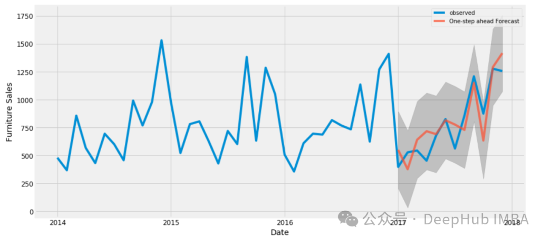
scheduler.step()训练后,表现最好的模型的训练损失为0.387,验证损失为0.457。当应用于测试集时,该模型的RMSLE为0.416,比赛排名为第89位(前10%)。
更大的嵌入和更多的注意力头似乎可以提高性能,但最好的结果是用一个单独的Transformer 实现的,这表明在有限的数据下,简单是优点。当放弃整体打乱而选择局部打乱时,效果有所改善;引入轻微的时间偏差提高了预测的准确性。
Recommend
About Joyk
Aggregate valuable and interesting links.
Joyk means Joy of geeK