

Happy New Year: GPT in 500 lines of SQL - EXPLAIN EXTENDED at EXPLAIN EXTENDED
source link: https://explainextended.com/2023/12/31/happy-new-year-15/
Go to the source link to view the article. You can view the picture content, updated content and better typesetting reading experience. If the link is broken, please click the button below to view the snapshot at that time.

Happy New Year: GPT in 500 lines of SQL
This year, the talk of the town was AI and how it can do everything for you.
I like it when someone or something does everything for me. To this end, I decided to ask ChatGPT to write my New Year's post:
"Hey ChatGPT. Can you implement a large language model in SQL?"
"No, SQL is not suitable for implementing large language models. SQL is a language for managing and querying data in relational databases. Implementing a language model requires complex algorithms, large datasets, and often deep learning frameworks, which are beyond the capabilities of SQL."
It just proves that if you want something done right, you have to do it yourself.
Encouraged by this optimistic forecast, today we will implement a large language model in SQL.
Theory
While writing this post, I used the wonderful article GPT in 60 Lines of NumPy by Jay Mody. This article explains the inner workings of a GPT model much better than I can hope to do. Still, a little recap is in order.
What is a generative large language model from a technical perspective?
A generative LLM is a function. It takes a text string as input (called "prompt" in AI parlance), and returns an array of strings and numbers. Here's what the signature of this function looks like:
llm(prompt: str) -> list[tuple[str, float]]
This function is deterministic. It does a lot of math under the hood, but all this math is hardwired. If you call it repeatedly with the same input, it will always return the same output.
It may come as a surprise to anyone who's been using ChatGPT and similar products because they can give different answers to the same question. Yet, it's true. We will shortly see how it works.
What are the values this function returns?
Something like this:
llm("I wish you a happy New")0 (' Year', 0.967553)1 (' Years', 0.018199688)2 (' year', 0.003573329)3 (' York', 0.003114716)4 (' New', 0.0009022804)…50252 (' carbohyd', 2.3950911e-15)50253 (' volunte', 2.2590102e-15)50254 ('pmwiki', 1.369229e-15)50255 (' proport', 1.1198108e-15)50256 (' cumbers', 7.568147e-17) |
It returns an array of tuples. Each tuple consists of a word (or, rather, a string) and a number. The number is the probability that this word will continue the prompt. The model "thinks" that the phrase "I wish you a happy New" will be followed by the character sequence " Year" with a probability of 96.7%, " Years" of 1.8% and so on.
The word "think" above is quoted because, of course, the model doesn't really think. It mechanically returns arrays of words and numbers according to some hardwired internal logic.
If it's that dumb and deterministic, how can it generate different texts?
Large language models are used in text applications (chatbots, content generators, code assistants etc). These applications repeatedly call the model and select the word suggested by it (with some degree of randomness). The next suggested word is added to the prompt and the model is called again. This continues in a loop until enough words are generated.
The accrued sequence of words will look like a text in a human language, complete with grammar, syntax and even what appears to be intelligence and reasoning. In this aspect, it is not unlike a Markov chain which works on the same principle.
The internals of a large language model are wired up so that the next suggested word will be a natural continuation of the prompt, complete with its grammar, semantics and sentiment. Equipping a function with such a logic became possible through a series of scientific breakthroughs (and programming drudgery) that have resulted in the development of the family of algorithms known as GPT, or Generative Pre-trained Transformer.
What does "Generative Pre-trained Transformer" mean?
"Generative" means that it generates text (by adding continuations to the prompt recursively, as we saw earlier).
"Transformer" means that it uses a particular type of neural network, first developed by Google and described in this paper.
"Pre-trained" is a little bit historical. Initially, the ability for the model to continue text was thought of as just a prerequisite for a more specialized task: inference (finding logical connections between phrases), classification (for instance, guessing the number of stars in a hotel rating from the text of the review), machine translation and so on. It was thought that these two parts should have been trained separately, the language part being just a pre-training for a "real" task that would follow.
As the original GPT paper puts it:
We demonstrate that large gains on these tasks can be realized by generative pre-training of a language model on a diverse corpus of unlabeled text, followed by discriminative fine-tuning on each specific task.
It was not until later that people realized that, with a model large enough, the second step was often not necessary. A Transformer model, trained to do nothing else than generate texts, turned out to be able to follow human language instructions that were contained in these texts, with no additional training ("fine-tuning" in AI parlance) required.
With that out of the way, let's focus on the implementation.
Generation
Here is what happens when we try to generate text from the prompt using GPT2:
def generate(prompt: str) -> str:# Transforms a string into a list of tokens.tokens = tokenize(prompt) # tokenize(prompt: str) -> list[int]while True:# Runs the algorithm.# Returns tokens' probabilities: a list of 50257 floats, adding up to 1.candidates = gpt2(tokens) # gpt2(tokens: list[int]) -> list[float]# Selects the next token from the list of candidatesnext_token = select_next_token(candidates)# select_next_token(candidates: list[float]) -> int# Append it to the list of tokenstokens.append(next_token)# Decide if we want to stop generating.# It can be token counter, timeout, stopword or something else.if should_stop_generating():break# Transform the list of tokens into a stringcompletion = detokenize(tokens) # detokenize(tokens: list[int]) -> strreturn completion |
Let's implement all these pieces one by one in SQL.
Tokenizer
Before a text can be fed to a neural network, it needs to be converted into a list of numbers. Of course, that's barely news: that's what text encodings like Unicode do. Plain Unicode, however, doesn't really work well with neural networks.
Neural networks, at their core, do a lot of matrix multiplications and capture whatever predictive powers they have in the coefficients of these matrixes. Some of these matrixes have one row per every possible value in the "alphabet"; others have one row per "character".
Here, the words "alphabet" and "character" don't have the usual meaning. In Unicode, the "alphabet" is 149186 characters long (this is how many different Unicode points there are at the time of this writing), and a "character" can be something like this: ﷽ (yes, that's a single Unicode point number 65021, encoding a whole phrase in Arabic that is particularly important for the Muslims). Note that the very same phrase could have been written in usual Arabic letters. It means that the same text can have many encodings.
As an illustration, let's take the word "PostgreSQL". If we were to encode it (convert to an array of numbers) using Unicode, we would get 10 numbers that could potentially be from 1 to 149186. It means that our neural network would need to store a matrix with 149186 rows in it and perform a number of calculations on 10 rows from this matrix. Some of these rows (corresponding to the letters of the English alphabet) would be used a lot and pack a lot of information; others, like poop emoji and obscure symbols from dead languages, would hardly be used at all, but still take up space.
Naturally, we want to keep both these numbers, the "alphabet" length and the "character" count, as low as possible. Ideally, all the "characters" in our alphabet should be distributed uniformly, and we still want our encoding to be as powerful as Unicode.
The way we can do that, intuitively, is to assign unique numbers to sequences of words that occur often in the texts we work with. In Unicode, the same religious phrase in Arabic can be encoded using either a single code point, or letter by letter. Since we are rolling our own encoding, we can do the same for the words and phrases that are important for the model (i.e. show up often in texts).
For instance, we could have separate numbers for "Post", "greSQL" and "ing". This way, the words "PostgreSQL" and "Posting" would both have a length of 2 in our representation. And of course, we would still maintain separate code points for shorter sequences and individual bytes. Even if we come across gibberish or a text in a foreign language, it would still be encodable, albeit longer.
GPT2 uses a variation of the algorithm called Byte pair encoding to do precisely that. Its tokenizer uses a dictionary of 50257 code points (in AI parlance, "tokens") that correspond to different byte sequences in UTF-8 (plus the "end of text" as a separate token).
This dictionary was built by statistical analysis performed like this:
- Start with a simple encoding of 256 tokens: one token per byte.
- Take a large corpus of texts (preferably the one the model will be trained on).
- Encode it.
- Calculate which pair of tokens is the most frequent. Let's assume it's 0x20 0x74 (space followed by the lowercase "t").
- Assign the next available value (257) to this pair of bytes.
- Repeat the steps 3-5, now paying attention to the byte sequences. If a sequence of bytes can be encoded with a complex token, use the complex token. If there are ambiguities (say, "abc" can, at some point, be encoded as "a" + "bc" or "ab" + "c"), use the one with the lowest number (because it was added earlier and hence is more frequent). Do this recursively until all sequences that can collapse into a single token will collapse into a single token.
- Perform the collapse 50000 times over.
The number 50000 was chosen more or less arbitrarily by the developers. Other models keep the number of tokens in a similar range (from 30k to 100k).
At every iteration of this algorithm, a new token that is a concatenation of two previous ones will be added to the dictionary. Ultimately, we will end up with 50256 tokens. Add a fixed-number token for "end-of-text", and we're done.
The GPT2 version of BTE has another layer of encoding: the token dictionary maps tokens to strings and not arrays of bytes. Mapping from bytes to string characters is defined in this function. We will save the dictionary it produces in the table encoder.
Let's see how we can implement the tokenizer in SQL.
The tokenizer is an integral part of GPT2, and the token dictionary can be downloaded from OpenAI's website along with the rest of the model. We will need to import it into the table tokenizer. At the bottom of this post, you will find a link to the code repository. Its code will automate populating database tables needed for the model.
In a recursive CTE, we will split this word into tokens (starting with single bytes) and merge the best adjacent pairs, until there is nothing left to merge. The merging itself happens in a nested recursive CTE.
For the demo, I will use the word "Mississippilessly". Each record in the resultset shows the best pair to collapse found so far, and also the progress through the query.
| step | token | combined | array_agg |
|---|---|---|---|
| 1 | None | None | ['M', 'i', 's', 's', 'i', 's', 's', 'i', 'p', 'p', 'i', 'l', 'e', 's', 's', 'l', 'y'] |
| 2 | 271 | is | ['M', 'is', 's', 'is', 's', 'i', 'p', 'p', 'i', 'l', 'e', 's', 's', 'l', 'y'] |
| 3 | 274 | es | ['M', 'is', 's', 'is', 's', 'i', 'p', 'p', 'i', 'l', 'es', 's', 'l', 'y'] |
| 4 | 306 | ly | ['M', 'is', 's', 'is', 's', 'i', 'p', 'p', 'i', 'l', 'es', 's', 'ly'] |
| 5 | 346 | il | ['M', 'is', 's', 'is', 's', 'i', 'p', 'p', 'il', 'es', 's', 'ly'] |
| 6 | 381 | pp | ['M', 'is', 's', 'is', 's', 'i', 'pp', 'il', 'es', 's', 'ly'] |
| 7 | 408 | ess | ['M', 'is', 's', 'is', 's', 'i', 'pp', 'il', 'ess', 'ly'] |
| 8 | 747 | iss | ['M', 'iss', 'iss', 'i', 'pp', 'il', 'ess', 'ly'] |
| 9 | 3974 | ipp | ['M', 'iss', 'iss', 'ipp', 'il', 'ess', 'ly'] |
| 10 | 17140 | Miss | ['Miss', 'iss', 'ipp', 'il', 'ess', 'ly'] |
| 11 | 30608 | iless | ['Miss', 'iss', 'ipp', 'iless', 'ly'] |
On each step, the BPE algorithm finds the best pair of tokens to merge and merges them (you can see the merged pair and its rank in the output). This procedure brings down the token space size from Unicode's 150k to 50k, and the number of tokens (in this particular word) from 17 to 5. Both are great improvements.
When working with multiple words, the tokenizer first splits the text into separate words using this regexp and merges the tokens inside each word separately. Unfortunately, PostgreSQL doesn't support Unicode character properties in regexps, so I had to tweak it a little bit (probably killing proper Unicode support in the process). Here's how it looks in SQL:
| token | cluster |
|---|---|
| 6307 | Post |
| 47701 | greSQL |
| 318 | Ġis |
| 1049 | Ġgreat |
The weird character Ġ is the whitespace.
This query tokenizes the prompt and converts it into an array of numbers. This way, the prompt is ready for its journey through the layers of the model.
Embeddings
The tokens represent parts of the human languages (about 0.75 words per token, in general), so any model that is trying to succeed at text completion should somehow encode the relationships between these parts. Even in isolation, the parts of the speech have sets of orthogonal properties.
Let's take the word "subpoena" (which happens to have a whole token in itself in the GPT2 tokenizer). Is it a noun? Yes, very much so. Is it a verb? Well, sort of. Is it an adjective? Not that much, but it can be if you squint hard enough. Is it legalese? Hell yes. And so on.
All these properties are orthogonal, i.e. independent of each other. A word can be a legalese noun but not an adjective or a verb. In English, any combination thereof can happen.
Things with orthogonal properties are best encoded using vectors. Instead of having a single property (like a token number), we can have many. And it helps if we can wiggle them as we want. For instance, for a word to continue the phrase "A court decision cited by the lawyer mentions the …" we would probably want something that's heavy on the legalese dimension and at the same time heavy on being a noun. We don't really care if it has a side hustle being an adjective, a verb, or a flower.
In math, mapping narrower values into wider spaces (such as token IDs to vectors) is called an embedding. This is exactly what we are doing here.
How do we decide which properties these vectors represent? We don't. We just provide enough vector space for every token and hope that the model during its training phase will populate these dimensions with something meaningful. GPT2 uses 768 dimensions for its vectors. There is no telling in advance (and, actually, even in the retrospective) what property of the word will, say, the dimension 247 encode. Surely it would encode something, but it's not easy to tell what it is.
What properties of each token do we want to embed in the vector space? Anything that has any bearing on what the next token would be.
Token id? Of course. Different tokens mean different things.
Position of the token in the text? Yes, please. "Blue violet" and "violet blue" are not the same thing.
Relationships of tokens to each other? Sure! That's, probably, the most important part of the job, and the Attention block of the Transformer architecture was the first one to get it right.
Tokens and positions are easy to embed. Let's say we have the phrase "PostgreSQL is great", which, as we already know, maps to four tokens: [6307, 47701, 318, 1049].
Among other parameters of GPT2, there are two matrixes called WTE (word token embedding) and WPE (word position embedding). As the names suggest, the former stores embeddings of the tokens, and the latter stores embeddings of the positions. The actual values of these embeddings have been populated ("learned") during the training of GPT2. As far as we are concerned, they are constants that live in the database tables wte and wpe.
WTE is 50257×768 and WPE is 1024×768. The latter means that the maximum number of tokens that we can use in a prompt to GPT2 is 1024. If we provide more tokens in the prompt, we just won't be able to pull positional embeddings for them. It's an architectural aspect ("hyperparameter" in AI parlance) of the model that is set at design time and cannot be changed by training. When people talk about the "context window" of an LLM, they mean this number.
We have the token 6307 at place 0, 47701 at 1, 318 at 2, and 1049 at 3. For each of these tokens and positions, we have two vectors: one from WTE and another one from WPE. We need to add them together. The four resulting vectors will be the inputs for the next part of the algorithm: the feed-forward neural network with the attention mechanism.
For the SQL part, we will use pgvector, a PostgreSQL extension.
A little disclaimer: normally, I write code for my New Year posts in vanilla SQL, sometimes with pure SQL functions as helpers. It would be perfectly possible to do it for this post as well by defining vector operations on arrays, at the cost of some performance decrease (it was done in version 1 and worked, albeit slowly). With the advent of the AI and growing importance of vector databases, pgvector or its equivalent will definitely make it into the core of PostgreSQL within two or three releases. I just decided to ride the wave of the future.
Here's how we do that in SQL:
WITH embeddings AS(SELECT place, valuesFROM UNNEST(ARRAY[6307, 47701, 318, 1049]) WITH ORDINALITY AS tokens (token, ordinality)CROSS JOIN LATERAL(SELECT ordinality - 1 AS place) oCROSS JOIN LATERAL(SELECT wte.values + wpe.values AS valuesFROM wteCROSS JOINwpeWHERE wte.token = tokens.tokenAND wpe.place = o.place) embedding)SELECT place, (values::REAL[])[0:5]FROM embeddings |
| place | values |
|---|---|
| 0 | [0.1035146, -0.22879261, 0.18413992, -0.29924694, 0.18642524] |
| 1 | [0.10757777, -0.0011023134, -0.0077463835, 0.03656415, -0.14654925] |
| 2 | [-0.005507436, -0.07471258, 0.11009377, -0.11708109, -0.14026159] |
| 3 | [-0.04785268, -0.0792546, 0.1628486, -0.3598496, 0.11462127] |
(To keep the output short, this query only shows the first 5 dimensions for each vector)
Attention
The part that really makes the Transformer architecture tick is the self-attention mechanism. It was first described in the 2017 paper "Attention is all you need" by Vasmani et al., probably the most famous AI paper, whose name has since become a snowclone (a cliché for naming other papers).
So far, we have several vectors that, hopefully, encode some syntactic and semantic properties of the words in our prompt. We need these properties to somehow transfer to the last vector. A little spoiler alert: at the end of the day, it will be the last vector that will store the embedding for the continuation word.
In a phrase like "I looked at the violet and saw that it was not the usual …", the ellipsis has to be something you see (and this notion has to jump from "saw"), something that's a property of a violet (jumping from "violet" to "it" and then to the ellipsis), and something that is "unusual" (jumping from "not" and "usual" and flipping the sign in the dimensions responsible for the usualness). The analogy in the real world would be a person reading a book in a foreign language that they kind of have a basic command of, but don't quite know very well. They would need to consciously trace their way from one word to another, and if they don't pay attention to the crucial part of the phrase, their understanding would be wrong.
To enable this transfer of meaning from one token to another, we need to allow the vectors of all the tokens to influence each other. If we want to populate the word "it" with some concrete semantics, how much of the semantics should come from the previous vectors in the prompt, and how much should remain from the word "it" itself?
To solve this problem, the model uses 12 sets of matrixes called Q (query), K (key) and V (value). Each of them has 64 columns. They are obtained from the vector embeddings through a 768×2304 linear transformation c_attn, whose weights and biases are stored in the tables c_attn_w and c_attn_b.
The result of c_attn is a matrix with n_token rows and 2304 columns (3×12×64). It consists of 12 Q matrixes, 12 K matrixes and 12 V matrixes stacked horizontally, in this order.
Each set of Q, K and V is called a "head". They are used to perform the step known as "multi-headed causal self-attention", by calculating the attention function.
Here's the formula for the attention function:
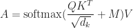
where softmax is the weight normalization function. It's defined like this:
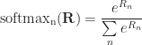

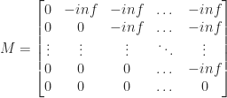
Softmax turns negative infinities into zeros.
Why do we need masking?
The prompt in our previous examples had 4 tokens, and the first thing the model did was calculate the 4 embeddings for these 4 tokens. As the model progresses, these vectors will undergo a lot of calculations, but for the most part, they will be independent and parallel. Changes in one vector will not affect the other vectors, as if they had not existed. The self-attention block is the only place in the whole model where the vectors affect each other.
Once the model is done with the math, the candidates for the next token will be decided solely from the last embedding. All the information flow should be directed towards this last vector and not from it. The transient values of the last embedding should not affect the transient values of the previous embeddings during the forward pass of the model.
That's why we "mask" the latter embeddings so that they don't influence the earlier embeddings through this particular channel. Hence the word "causal" in "multi-headed causal self-attention".
Why are the matrixes called "query", "key" and "value"?
To be honest, I'm not sure it's even a good analogy. But I'll still do my take on the intuition behind it.
In machine learning, generally, calculations should not involve variable-length loops or statement branching. Everything should be done through the composition of simple analytic functions (additions, multiplications, powers, logarithms and trig). It allows backpropagation, which relies on technologies like automatic differentiation, to work efficiently.
The mathematical model of the key-value store is the expression
, but it's not a smooth, differentiable function and it will not work well with backpropagation. To make it work, we would need to turn it into a smooth function that would be close to 


The Gaussian distribution ("bell curve"), scaled to

, where 
In a vector space with many enough dimensions, if we take a fixed vector 


Again, this analogy is far-fetched. It's best not to pay too much attention (no pun intended) to these concepts of attention, meaning flow, hash tables and so on. Just think of them as an inspiration for a math trick that has been put to the test and proved to work really well.
Let's illustrate this step:
| place | q | k | v | matrix | attention |
|---|---|---|---|---|---|
| 0 | +0.381 -0.579 +0.073 … | -1.395 +2.367 +0.332 … | -0.006 +0.192 +0.047 … | 1.00 0 0 0 | -0.006 +0.192 +0.047 … |
| 1 | +1.518 +0.827 -0.388 … | -2.380 +3.714 +0.659 … | -0.315 -0.062 +0.018 … | 0.73 0.27 0 0 | -0.089 +0.124 +0.039 … |
| 2 | +0.238 -0.226 +0.344 … | -1.952 +2.404 +1.953 … | +0.256 -0.268 +0.301 … | 0.67 0.26 0.07 0 | -0.069 +0.095 +0.057 … |
| 3 | +1.130 -0.011 -0.103 … | -2.855 +2.053 +2.813 … | +0.176 +0.019 -0.099 … | 0.59 0.19 0.12 0.10 | -0.016 +0.071 +0.058 … |
Here is what we did:
- Before calculating the attention function, we normalized the vectors by applying the linear transformation
. The matrix
and the vector
are called "scale" and "shift", accordingly. They are learned parameters of the model, which are stored in the tables
ln_1_gandln_1_b - We are only showing the first head of the first layer of the algorithm. After we multiplied the vectors by the learned coefficients from
c_attn_wandc_attn_b("weight" and "bias"), we sliced the resulting 2304-vectors, taking 64-vectors starting at the positions 0, 768 and 1536. They correspond to the vectors Q, K and V for the first head. EXPin PostgreSQL fails on really small numbers, that's why we shortcut to zero if the argument toEXPis less than -745.13.- We are only showing the first three elements for each vector. The attention matrix we show in full.
As we can see, the first value vector got copied to the output as is (as it will do in every other layer of the algorithm). It means that once the model has been trained, the output embedding for the first token will be only defined by the value of the first token. In general, during the recursive inference phase, where tokens only get added to the prompt, only the last embedding in the output will ever change compared to the previous iteration. This is what the causal mask does.
Looking a bit forward: the attention block is the only place in the entire algorithm where tokens can influence each other during the forward pass. Since we have disabled the ability of later tokens to influence the previous ones in this step, all the calculations done on the previous tokens can be reused between the forward passes of the model.
Remember, the model operates by appending tokens to the prompt. If our original (tokenized) prompt is "Post greSQL Ġis Ġgreat" and the next one will be (for instance) "Post greSQL Ġis Ġgreat Ġfor", all the results of the calculations made on the first four tokens can be reused for the new prompt; they will never change, regardless of what is appended to them.
Jay Mody's illustrative article doesn't make use of this fact (and neither do we, for the sake of simplicity), but the original GPT2 implementation does.
Once all the heads are done, we will end up with 12 matrixes, each 64 columns wide and n_tokens rows tall. To map it back to the dimension of embedding vectors (768), we just need to stack these matrixes horizontally.
The final step of multi-headed attention involves projecting the values through a learned linear transformation of the same dimension. Its weights and biases are stored in the tables c_proj_w and c_proj_b.
Here's what the code for a complete multi-headed attention step in the first layer looks like:
| place | q |
|---|---|
| 0 | +0.814 -1.407 +0.171 +0.008 +0.065 -0.049 -0.407 +1.178 -0.234 -0.061 … |
| 1 | +1.150 -0.430 +0.083 +0.030 +0.010 +0.015 -0.245 +3.778 -0.445 -0.004 … |
| 2 | -0.219 -0.745 -0.116 +0.032 +0.064 -0.044 +0.290 +3.187 -0.074 -0.003 … |
| 3 | -0.526 -0.757 -0.510 -0.008 +0.027 -0.017 +0.302 +2.842 +0.188 -0.028 … |
Before the results of multi-headed attention are passed to the next step, the original inputs are added to them. This trick was described in the original transformer paper. It's supposed to help with vanishing and exploding gradients.
It's a common problem during training: sometimes the gradients of the parameters turn out too big or too small. Changing them on the training iteration either has very little effect on the loss function (and so the model converges very slowly), or, on the opposite, has such a big effect that even a small change throws the loss function too far away from its local minimum, negating the training efforts.
Feedforward
This is what the deep neural networks do. The larger part of the model parameters is actually used at this step.
This step is a multi-layer perceptron with three layers (768, 3072, 768), using the Gaussian Error Linear Unit (GELU) as an activation function:


This function has been observed to yield good results in deep neural networks. It can be analytically approximated like this:
![\mathrm{GELU}(x) \displaystyle \approx 0.5x \left(1 + \mathrm{tanh}\left[0.797884\left(x + 0.044715x^3\right) \right]\right)](https://s0.wp.com/latex.php?latex=%5Cmathrm%7BGELU%7D%28x%29+%5Cdisplaystyle+%5Capprox+0.5x+%5Cleft%281+%2B+%5Cmathrm%7Btanh%7D%5Cleft%5B0.797884%5Cleft%28x+%2B+0.044715x%5E3%5Cright%29+%5Cright%5D%5Cright%29+&bg=fff&fg=1c1c1c&s=0&c=20201002)
The learned linear transformation parameters for layer connections are called c_fc (768 → 3072) and c_proj (3072 → 768). The values for the first layer are first normalized using the coefficients in the learned parameter ln_2. After the feedforward step is completed, its input is again added to the output. This, too, is a part of the original transformer design.
The whole feedforward step looks like this:

And here's how we do this in SQL:
| place | q |
|---|---|
| 0 | +0.309 -1.267 -0.250 -1.111 -0.226 +0.549 -0.346 +0.645 -1.603 -0.501 … |
| 1 | +0.841 -1.081 +0.227 -1.029 -1.554 +1.061 -0.070 +5.258 -1.892 -0.973 … |
| 2 | -1.256 -0.528 -0.846 -0.288 +0.166 +0.409 +0.019 +3.393 +0.085 -0.212 … |
| 3 | -1.007 -1.719 -0.725 -1.417 -0.086 -0.144 +0.605 +3.272 +1.051 -0.666 … |
This output is what comes out of the first block of GPT2.
Blocks
What we saw in the previous steps is repeated in layers (called "blocks"). The blocks are set up in a pipeline so that the output of a previous block goes straight to the next one. Each block has its own set of learned parameters.
In SQL, we would need to connect the blocks using a recursive CTE.
Once the final block produces the values, we need to normalize it using the learned parameter ln_f.
Here's what the model ultimately looks like:


![\displaystyle \mathbf R_0 = \mathrm{wte}(tokens) + \mathrm{wpe}([1 \ldots \mathrm{dim}(tokens)])](https://s0.wp.com/latex.php?latex=%5Cdisplaystyle+%5Cmathbf+R_0+%3D+%5Cmathrm%7Bwte%7D%28tokens%29+%2B+%5Cmathrm%7Bwpe%7D%28%5B1+%5Cldots+%5Cmathrm%7Bdim%7D%28tokens%29%5D%29&bg=fff&fg=1c1c1c&s=0&c=20201002)
And here's how it looks in SQL:
| place | q |
|---|---|
| 0 | -0.153 -0.126 -0.368 +0.028 -0.013 -0.198 +0.661 +0.056 -0.228 -0.001 … |
| 1 | -0.157 -0.314 +0.291 -0.386 -0.273 -0.054 +3.397 +0.440 -0.137 -0.243 … |
| 2 | -0.912 -0.220 -0.886 -0.661 +0.491 -0.050 +0.693 +1.128 +0.031 -0.577 … |
| 3 | -0.098 -0.323 -1.479 -0.736 +0.235 -0.608 +1.774 +0.566 -0.057 -0.211 … |
This is the output of the model.
The fourth vector is the actual embedding of the next token predicted by the model. We just need to map it back to the tokens.
Tokens
We have an embedding (a 768-vector) which, according to the model, captures the semantics and the grammar of the most likely continuation of the prompt. Now we need to map it back to the token.
One of the first steps the model makes is mapping the tokens to their embeddings. It is done through the 50257×768 matrix wpe. We will need to use the same matrix to map the embedding back to the token.
The problem is that the exact reverse mapping is not possible: the embedding will not (likely) be equal to any of the rows in the matrix. So we will need to find the "closest" token to the embedding.
Since the dimensions of embeddings capture (as we hope) some semantic and grammatical aspects of the token, we need them to match as closely as possible. One way to consolidate the closeness of each dimension would be to just calculate the dot product of the two embeddings. The higher the dot product, the closer the token is to the prediction.
To do this, we will multiply the embedding by the matrix wte. The result will be a single-column matrix, 50257 rows tall. Each value in this result will be the dot product of the predicted embedding and the token embedding. The higher this number, the more likely it is for the token to continue the prompt.
To pick the next token, we will need to convert the similarities to probabilities. To do this, we will use our good friend softmax (the same function that we used to normalize attention weights).
Why use softmax for probabilities?
Softmax has the nice property of satisfying Luce's choice axiom. It means that the relative probabilities of two options don't depend on the presence or probability of other options. If A is twice as probable as B, then the presence or absence of other options will not change this ratio (although it of course can change the absolute values).
The vector of dot products ("logit" in AI parlance) contains arbitrary scores that don't have an intrinsic scale. If A has a larger score than B, we know that it's more likely, but that's about it. We can tweak the inputs to softmax as we please, as long as they keep their order (i.e. larger scores stay larger).
One common way to do that is to normalize the scores by subtracting the greatest value from the set from them (so that the biggest score becomes 0 and the rest become negative numbers). Then we take some fixed number (let's say five or ten) top scores. Finally, we multiply each score by a constant before feeding it to softmax.
The number of top scores that we take is usually called 

The formula for tokens' probabilities is 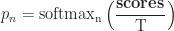

Why is it called "temperature"?
The softmax function has another name: Boltzmann distribution. It's extensively used in physics. Among other things, it serves as a base for the barometric formula, which tells how density or air varies with altitude.
Intuitively, hot air rises. It spreads further away from the Earth. When air is hot, it's more likely for an air molecule to bounce off its neighbors and jump at an otherwise impossible height. Compared to colder temperatures, air density increases at higher altitudes and drops at sea level.
See how air behaves at different temperatures:
Courtesy of Dominic Ford, Bouncing Balls and the Boltzmann Distribution
By analogy, a large "temperature" increases the probability of second-choice tokens being selected (at the expense of the first-choice tokens, of course). The inference becomes less predictable and more "creative".
Let's put this all into SQL. The prompt was "PostgreSQL is great". Here are the top 5 tokens that, according to the model, are most likely to continue this phrase, and their probabilities at different temperatures:
| token | cluster | score | temperature = 0.5 | temperature = 1 | temperature = 2 |
|---|---|---|---|---|---|
| 329 | Ġfor | -85.435 | 0.74 | 0.48 | 0.33 |
| 11 | , | -86.232 | 0.15 | 0.22 | 0.22 |
| 13 | . | -86.734 | 0.05 | 0.13 | 0.17 |
| 379 | Ġat | -86.785 | 0.05 | 0.12 | 0.17 |
| 284 | Ġto | -87.628 | 0.01 | 0.05 | 0.11 |
Inference
Finally, we are ready to do some real inference: run the model, select a token according to its probability, add it to the prompt and repeat until enough tokens are generated.
The LLM itself, as we saw before, is deterministic: it's just a series of matrix multiplications and other math operations on predefined constants. As long as the prompt and the hyperparameters like temperature and top_n are the same, the output will also be the same.
The only non-deterministic process is token selection. There is randomness involved in it (to a variable degree). That's why GPT-based chatbots can give different answers to the same prompt.
We will use the phrase "Happy New Year! I wish" as the prompt and make the model generate 10 new tokens for this prompt. The temperature will be set to 2, and top_n will be set to 5.
The query runs for 2:44 minutes on my machine. Here's its output:
| response |
|---|
| Happy New Year! I wish you all the best in your new year! |
This part the AI got right. I do wish you all the best in your new year!
You can find the queries and the installation code in the GitHub repository: quassnoi/explain-extended-2024
Previous New Year posts:
Recommend
About Joyk
Aggregate valuable and interesting links.
Joyk means Joy of geeK