

Cellular Automata Using Rust: Part I
source link: https://xebia.com/blog/cellular-automata-using-rust-part-i/
Go to the source link to view the article. You can view the picture content, updated content and better typesetting reading experience. If the link is broken, please click the button below to view the snapshot at that time.
Cellular Automata Using Rust: Part I

In this three-part series and the associated project, we are going to bring elementary cellular automata to life using the Rust programming language and the Bevy game engine. We'll learn a few things about cellular automata, Rust, entity-component-system architecture, and basic game development. You can experiment with the finished web app online; just give your browser a moment to download the app, and click the grid to give the app focus.
A cellular automaton comprises a regular grid of cells, each of which must express exactly one of a finite set of states. For each cell, it and its adjacent cells constitute its neighborhood; to avoid edge conditions herein, we choose to consider that the two "edges" of each dimension are adjacent. A cellular automaton may occupy an arbitrary, nonzero number of dimensions, and each dimension is considered for the purpose of identifying a cell's neighborhood. A cellular automaton evolves over time as governed by some rule that dictates the next state of each cell based on the current state of its neighborhood. The full set of next states is called the next generation. The evolutionary rule is typically uniform and unchanging over time, but this is not strictly required; in particular, in our project we let the user pause the simulation to change rules and even manually toggle cell states.
We're in this for the fun of watching cellular automata evolve, but cellular automata are more than mere mathematical toys. They showcase how complex behavior can arise naturally from minimal state and simple rules. In particular, Rule #110 is Turing-complete, able to implement a universal cyclic tag system that can emulate any Turing machine.
This elegance has drawn great minds for decades. Stanisław Ulam and John von Neumann discovered cellular automate in the 1940s during their time together at Los Alamos National Laboratory. In 1970, John Conway introduced the Game of Life, the two-dimensional cellular automaton now famous for its blocks, beehives, boats, blinkers, pulsars, gliders, and spaceships. In 1982, Conway published a proof of Turing-completeness, finally putting the automaton on the same computational footing as Turing machines and lambda calculus. Also in the 1980s, Stephen Wolfram published A New Kind of Science, wherein he systematically studied elementary cellular automata — one-dimensional cellular automata of irreducible simplicity. In 1985, Wolfram first conjectured that Rule #110 was Turing-complete, and in 2004, Matthew Cook published the proof.
Elementary cellular automata
An elementary cellular automaton is usually conceptualized as a single row of
cells, each of which must express one of two states: on, represented by a
black cell; or off, represented by a white cell. If you're already familiar
with the Game of Life, then you might think of on as live and off as dead. But the Game of Life, being two-dimensional, is not an elementary
cellular automaton, so we're moving on without it.
Multiple generations are usually represented as a two-dimensional grid, such that each row represents a complete generation. New generations are added at the end, so evolution progresses downward over time. Note that these are arbitrary choices of convenience to support visualization over time, not essential properties of the abstract automaton. To better study the complexity-from-simplicity phenomenon, evolution is frequently driven by a single fixed rule. This rule encodes the complete transition table for the eight possible neighborhoods.
To see why there are eight possible neighborhoods, let's consider adjacency in one-dimensional space. We'll define the distance between two cells 𝑎 and 𝑏 in the natural way: as the number of cell borders that must be crossed in transit from 𝑎 to 𝑏. Further, we'll define the neighborhood of some cell 𝑎 as comprising all cells whose distance from 𝑎 is less than or equal to one. For any cell 𝑎, that gives us 𝑎's left neighbor, 𝑎 itself, and 𝑎's right neighbor. It follows that each cell is considered three times — once as the center, once as the left neighbor, and once as the right neighbor.
Now recall that each cell can express exactly two states, on and off. Taking
state into account, there are a total of 2³ = 8 possible neighborhoods. Using X to represent on and • to represent off, the eight possible
neighborhoods and their population ordinals are:
••• (0)
••X (1)
•X• (2)
•XX (3)
X•• (4)
X•X (5)
XX• (6)
XXX (7)A rule dictates the outcome — on or off — for each cell as a consequence of
its previous neighborhood state. Because there are eight possible neighborhoods,
and each neighborhood can produce one of two resultant states, there are 2⁸ =
256 possible rules. The result state of each neighborhood can be mapped to a
single bit in an 8-bit number; this representational strategy is commonly called Wolfram coding. In a Wolfram code, each bit, numbered 0 through 7,
corresponds to one of the eight possible neighborhoods illustrated above. The
presence of a 1 in the 𝑛th bit means that neighborhood 𝑛 produces an on cell, whereas 0 at 𝑛 means that the neighborhood produces an off cell.
Let's consider Rule #206 as a concrete case. First, we convert to binary to obtain:

We can visualize the transition table thus:
                         Rule #206
bit index  =    7     6     5     4     3     2     1     0
binary     =    1     1     0     0     1     1     1     0
input      =   XXX   XX•   X•X   X••   •XX   •X•   ••X   •••
output = X X • • X X X •For convenience of demonstration only, we restrict the cellular automaton to 30
cells. We are free to choose an initial generation for our cellular automaton
arbitrarily, though certain choices lead to much more interesting results.
Because it will be interesting, we begin with only one cell expressing the on state. Then we run Rule #206 for 9 generations.
generation  1 = •••••••••••••••X••••••••••••••
generation  2 = ••••••••••••••XX••••••••••••••
generation  3 = •••••••••••••XXX••••••••••••••
generation  4 = ••••••••••••XXXX••••••••••••••
generation  5 = •••••••••••XXXXX••••••••••••••
generation  6 = ••••••••••XXXXXX••••••••••••••
generation  7 = •••••••••XXXXXXX••••••••••••••
generation  8 = ••••••••XXXXXXXX••••••••••••••
generation  9 = •••••••XXXXXXXXX••••••••••••••
generation 10 = ••••••XXXXXXXXXX••••••••••••••Two cool things happened here. One is easy to see, literally: it drew a right
triangle. The other requires a bit of interpretation. We've relied on binary
codings a lot already in this post, so let's indulge a bit more. We can treat
the on cells as a string of binary digits, such that the rightmost on cell
corresponds to 20. Now we can interpret the generations as the elements in a
sequence:
1, 3, 7, 15, 31, 127, 511, 2047, 8191, 32767, …This series corresponds to the Mersenne numbers, where 𝑛 >= 1:
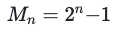
Other rules produce evolutions with startling correspondences to other mathematical entities, like the Jacobsthal numbers and Pascal's triangle. And rules #110 and #124 are both capable of universal computation.
Now that we know what elementary cellular automata are and why they might be interesting, let's model them in Rust.
Modeling Elementary Cellular Automata with Rust
There's a project based on this blog post. It's laid out in a pretty vanilla fashion, completely standard for a simple binary crate. When I present a code excerpt, I typically strip out any comments, but you can see all the original comments intact in the project on GitHub.
The data model for the elementary cellular automaton is in src/automata.rs, so all the code excerpts in this
section are sourced from that file.
Let's look at the representation of an elementary cellular automaton first.
Automaton, const genericity, and conditional derivation
Essentially, we keep our representational strategy super simple: we express an elementary cellular automaton as a boolean array, albeit with a few elegant frills, like conditional derivation for testing.
#[derive(Copy, Clone, Debug)]
#[cfg_attr(test, derive(PartialEq, Eq))]
pub struct Automaton<const K: usize = AUTOMATON_LENGTH>([bool; K]);
Using the newtype pattern, we define a 1-element tuple struct to wrap an
array of K booleans. Rather than hard coding the exact size, we offer some
flexibility through const generics. In Rust, const genericity ranges over
values of primitive types rather than types or lifetimes. We default the const parameter to AUTOMATON_LENGTH, making the bare type Automaton equivalent to Automaton. Elsewhere, we establish AUTOMATON_LENGTH itself:
pub const AUTOMATON_LENGTH: usize = 64;Because AUTOMATON_LENGTH is const data, we can use it to satisfy the const parameter K. So our default Automaton will comprise 64 cells, which is
plenty for an interesting visualization.
bool implements Copy, and arrays implement Copy if their element type
does. Extending this chain of reasoning to structs, tuples, and struct
tuples, our newtype is also eligible to implement Copy because its only field
implements Copy. Even if we changed AUTOMATON_LENGTH to some other number,
it would need to be small enough to support all-at-once presentation in the
application, so it's efficient enough to derive Copy for Automaton.
The application itself doesn't rely on comparison, but the test suite does. We
get the best of both worlds with cfg_attr: we implement PartialEq and Eq only when compiling and linking the test suite.
Note that the natural ordering of the cells within the Automaton tracks the
array itself, so the cell at index 0 is the leftmost cell and the cell at
index K - 1 is the rightmost cell. This will matter several times, because
different contexts imply different natural orderings, and we will sometimes need
to perform coordinate transformations to account for this.
Succession and const fn
Now let's look at the next method that computes the next generation of an Automaton. There are three cases that next needs to handle:
- Computing the leading edge cell, i.e., the rightmost one, which requires treating the trailing edge cell, i.e., the leftmost one, as its right neighbor. In other words, we visualize the automaton as a row, but we treat it like a ring that wraps around at the ends.
- Computing the medial cells, which is trivial once we are properly oriented.
- Computing the trailing edge cell, which requires treating the leading edge cell as its left neighbor.
impl<const K: usize> Automaton<K>
{
    pub fn next(&self, rule: AutomatonRule) -> Self
    {
        let mut next = [false; K];
        // Compute the leading edge cell, treating the final cell of the
        // automaton as its right neighbor.
        let ordinal = compute_ordinal(self[1], self[0], self[K - 1]);
        next[0] = rule.next_cell(ordinal);
        // Computing the medial cells is trivial.
        for i in 1 ..= K - 2
        {
            let ordinal = compute_ordinal(
                self[i + 1],
                self[i],
                self[i - 1]
            );
            next[i] = rule.next_cell(ordinal);
        }
        // Compute the trailing edge cell, treating the initial cell of the
        // automaton as its left neighbor.
        let ordinal = compute_ordinal(self[0], self[K - 1], self[K - 2]);
        next[K - 1] = rule.next_cell(ordinal);
        Automaton(next)
    }
}
compute_ordinal is a const function that determines the population ordinal
for some cell's neighborhood. To keep it independent of any particular cell's
identity, it accepts the exploded neighborhood state and answers the population
ordinal.
#[inline]
const fn compute_ordinal(left: bool, middle: bool, right: bool) -> u8
{
    let left = if left { 4u8 } else { 0 };
    let middle = if middle { 2u8 } else { 0 };
    let right = if right { 1u8 } else { 0 };
    let ordinal = left | middle | right;
    // Note that we cannot test range containment directly here because
    // `contains` is not a `const fn`.
    assert!(ordinal <= 7);
    ordinal
}
By the way, a const function can be used at compile time to initialize const data. Const Rust is a foldable subset of Rust that operates only on literals, const data, and values produced by const functions. The compiler evaluates and folds const expressions down into a single result. Using const functions lets your initialization logic focus on semantics rather than magic numbers. Const Rust is still limited in scope — it can't handle loops yet, for example — but it has steadily gained more features over many releases. A good rule of thumb is to make data and functions const wherever possible, as it expands your compile-time vocabulary and thus improves the expressiveness of your const and static initializers.
Right, back to next. Armed with the population ordinal, we can call the next_cell method (shown below) to ask the supplied rule to produce the
appropriate successor for the corresponding neighborhood. After that, it's
simply a matter of clobbering the slots of the eponymous next array, then
wrapping an Automaton around it before returning.
Rules
AutomataRule represents an evolutionary rule, once again using the newtype
pattern. This newtype wraps a Wolfram code, expressed as a u8.
#[derive(Copy, Clone, Default, Debug, PartialEq, Eq, PartialOrd, Ord, Resource)]
pub struct AutomatonRule(u8);
ResourcetraitNote: We derive a bunch of standard Rust traits here, but
Resourcestands out as something different.Resourceis a derivable trait provided by Bevy, denoting a type that can be used as a global resource. More on this in the next blog post.

Now we look at next_cell, which is completely straightforward:
impl AutomatonRule
{
    #[inline]
    const fn next_cell(self, ordinal: u8) -> bool
    {
        self.0 & (1 << ordinal) != 0
    }
}
Recall that the Wolfram code specifies the complete transition table for an elementary cellular automaton using only eight bits, so it's a simple matter of extracting the bit associated with a population ordinal. It's just a bit shift, a bitwise and, and a test against zero.
Instantiating an Automaton
We need a clean way to populate an Automaton:
impl<const K: usize> From<u64> for Automaton<K>
{
    fn from(value: u64) -> Self
    {
        assert!(K <= 0u64.count_zeros() as usize);
        let mut next = [false; K];
        for i in 0 ..= K - 1
        {
            next[i] = value & (1 << i) != 0;
        }
        Automaton(next)
    }
}
Pretty straightforward. There are only a couple tricks here.
- We need to traverse both the array and the
u64in the same direction, i.e., from least-significant cell to most-significant cell. For the array, this means indexing up from zero; for theu64, this means masking up from 20 to 2(63). - The
assert!macro call is a dynamic guard on the value of the const parameterK.count_zerosis a const fn, which we use to obtain the number of bits in au64. We could instead insert the literal64, of course, but this technique clearly preserves the correlation between the type and its bit length. SinceKis a const parameter andcount_zerosis a const fn with a literal receiver (0u64), the whole predicate is a const expression, meaning that the compiler can optimize away the runtime check whenever the const expression evaluates totrue. In release mode, this ends up being a static guard after all!
Const implementation bounds
Note: const implementation bounds, i.e., const expressions in const parameter positions, are available in nightly Rust, but not in stable Rust. With the nightly toolchain, we could use a conditional trait implementation on an unrelated helper type to statically guard against out-of-range values of
Kthrough emission of a compiler error.
// Available in nightly only.
trait IsTrue {}
struct Guard<const C: bool>;
impl IsTrue for Guard<true> {}

impl<const K: usize> From<u64> for Automaton<K> where Guard<{K <= 64}>: IsTrue
{
    fn from(value: u64) -> Self
    {
        // …
    }
}
In this scenario, out-of-range
Kdisables the implementation ofFromforAutomaton, so attemptingfromwith, e.g., anAutomaton, causes the compiler to announce that the trait isn't implemented.But the
assert!technique is the best we can do with stable Rust, and we use stable Rust through this project in order to maximize stability and availability.
Testing the evolutionary mechanism
Before moving on to Bevy, we should test whether all
this works. We pick an arbitrary initial generation and rule, mechanically
perform an evolution by hand, then rely on structural induction to conclude that
the implementation is correct. Because we're free to pick anything we want, we
pick initial generation 0x34244103 and rule #110. We also choose a shorter
length automaton — 30 cells instead of 64 — for convenience. This scenario is illustrated on Wikipedia, so we can treat it as a community-checked test vector.
#[test]
fn rule_110()
{
    //     XX•X••••X••X•••X•••••X••••••XX
    // 0b00110100001001000100000100000011
    // 0x   3   4   2   4   4   1   0   3
    let automaton = Automaton::<30>::from(0x34244103);
    //     •XXX•••XX•XX••XX••••XX•••••XX•
    // 0b00011100011011001100001100000110
    // 0x   1   C   6   C   C   3   0   6
    let expected = Automaton::<30>::from(0x1C6CC306);
    let actual = automaton.next(110.into());
    assert_eq!(expected, actual);
}
Ring buffers and impl Trait syntax
We want to visualize more than one generation, however, because otherwise we can't experience any cool series or structures, like Sierpiński triangles. We want to see how a cellular automaton evolves over time, at least over the course of, say, fifty generations.
pub const AUTOMATON_HISTORY: usize = 50;To avoid excessive memory retention or having to accommodate a scrollable
viewport, we bound the evolution to AUTOMATON_HISTORY generations. We should
keep only the most recent generations, of course, with the current generation at
the frontier. A ring buffer seems like the natural choice to satisfy these
goals.
The crate ringbuffer provides a solid
implementation with a convenient API, so let's bring it into our project. We add
the following to our Cargo.toml:
[dependencies]
ringbuffer = "0.15.0"
Back in src/automata.rs, we introduce History as
another const-generic newtype, this one wrapping a ConstGenericRingBuffer:
#[derive(Debug, Resource)]
pub struct History<
    const K: usize = AUTOMATON_LENGTH,
    const N: usize = AUTOMATON_HISTORY
>(
    ConstGenericRingBuffer<Automaton<K>, N>
);
As strongly implied by its name, ConstGenericRingBuffer also uses const genericity, so it fits perfectly with our strategy. Thinking ahead to our UI, we
need to present an entire history, with perhaps a single active generation at
the tail. We could special case the UI setup logic, but since the memory for the
ring buffer is already committed, it's cleaner to pre-populate History with
empty automata.
impl<const K: usize, const N: usize> History<K, N>
{
    pub fn new() -> Self
    {
        let mut ring = ConstGenericRingBuffer::new();
        for _ in 0 .. N
        {
            ring.push(Automaton::default());
        }
        assert!(ring.is_full());
        Self(ring)
    }
}
ConstGenericRingBuffer::new builds an empty ring buffer, and our loop fills it
with empty automata. Fullness of the ring buffer is an essential postcondition
for our use case, so we assert! it for sincerity. Now we can iterate through
the history, from oldest to newest, and know that fifty generations will occur.
impl<const K: usize, const N: usize> History<K, N>
{
    pub fn newest(&self) -> &Automaton<K> { self.0.back().unwrap() }
    pub fn oldest(&self) -> &Automaton<K> { self.0.front().unwrap() }
    pub fn iter(&self) -> impl Iterator<Item=&Automaton<K>> { self.0.iter() }
}
We can safely unwrap in newest and oldest because we have ensured
fullness, which is a stronger precondition than nonemptiness, which is all that unwrap requires here.
But the most interesting thing here is the return type of iter, which employs
what Rust calls impl Trait syntax. The concrete iterator defined in the ringbuffer crate is called RingBufferIterator, and it is private to the
crate. We can't name this type at all in our own code, meaning that we can
neither directly mention it in a method signature nor encapsulate it inside
another type. impl Iterator declares that we return some concrete type that
implements the trait Iterator, but keeps the identity of that type vague. It
allows the private type to remain hidden, even to us, but still allows us to
re-export that type anonymously from our own API. This kind of ad hoc genericity is very useful at API boundaries, and more ergonomic than introducing
a named type parameter.
Evolving the automaton
Evolving the cellular automaton is just a simple matter of using the data and logic that we've already seen:
impl<const K: usize, const N: usize> History<K, N>
{
    pub fn evolve(&mut self, rule: AutomatonRule)
    {
        self.0.push(self.newest().next(rule));
    }
}
That's everything we need from the model, so it's time to leave src/automata.rs behind and turn our attention to the UI
— in the next blog post in this series.
Recommend
About Joyk
Aggregate valuable and interesting links.
Joyk means Joy of geeK