Pooling overdispersed binomial data to estimate event rate

Methods

The Beta-Binomial distribution

Both Chuang-Stein [2] and Ennis [5] provide excellent references for those who are interested in the history of the beta-binomial model. Recall the definition of the binomial distribution:

where x is the number of successes in a sequence of n independent success/failure experiments, each of which has probability p for success.

Let probability p follow a beta distribution (p|α, β), then

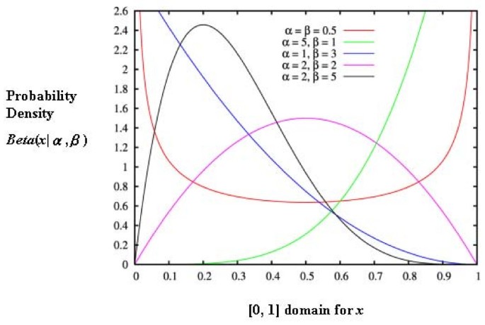
where Γ is the gamma function over the domain [0, 1]; α and β are two positive parameters. The beta distribution was selected in the past because of its flexibility (capable of a wide range of shapes, see Figure 1) and its ability to provide good approximations. As Skellam [8] stated as early as 1948, "in practice we could, at least in most cases, take this form of distribution as a convenient approximation." As a result, we arrive at a combination of the binomial distribution with a beta density function:

where x takes on the values 0, 1, 2... n, and α and β are positive. Note in equation (3) that n is the total number of study subjects, and x is the total number of subjects with a certain adverse event, although what most investigators are interested in is the proportion p that varies between 0 and 1 and has the appearance of a continuous distribution.

So let p i = x i /n i , i = 1,2, ... k, where i indexes the different studies, x i is the number of events in the ith study and n i is the sample size of the study. To reiterate, within the context of multiple studies where each study with sample size n i and binomial probability p i (e.g. for adverse events), one binomial distribution cannot adequately describe the additional variation when p i varies and thus the data are fitted with a beta distribution with parameters (α, β), with α > 0 and β > 0. Let μ = α/(α+β), θ = 1/(α+β), where μ is the mean event rate (i.e., the expected value of a variable binomial parameter p) and θ is a measure of the variation in p. In short, we have constructed a two-stage model:

X i | p i ~Bin(n i , p i )

p i ~Beta (μ, θ),i.i.d

The mean and variance of X are nμ and nμ(1-μ){θ/(1+θ)} [9]. One can view the term {θ/(1+θ)} as a multiplier of the binomial variance. In other words, it models the overdispersion. Some authors (e.g. Kleinman [10]) prefer the term γ where γ = θ/(1+θ) = 1/(α+β+1). Then the variance is nμ(1 - μ) γ. In essence, one can derive the same information from θ and γ about the beta-binomial distribution, so it is beneficial to know both and employ whichever is more convenient for computation.

Estimation of Parameters

Two main methods, one involving moments and the other involving maximum likelihood, are often used to estimate the parameters μ and θ.

The Moment Estimates Method

In terms of actual data observed from different studies, let p i = x i /n i , i = 1,2, ... k, where i indexes the different studies, x i is the number of events in the ith study and n i is the sample size of the study. The n i 's here are almost always unequal in clinical studies.

where {w i } represents a set of weights and w is the sum of all the weights [10].

Let also MathML

then the moment estimates of μ and γ are:

MathML and

where MathML. To derive θ, we can simply perform the following conversion:

θ = γ/(1 - γ)

Providing the proper set of weights is challenging because {w i } is a function of the unknown parameter γ. Kleinman [10] first offered an empirical weighting procedure and suggested to set w i = n i or w i = 1 to obtain an initial approximation of estimates of μ and γ using equation (4). Using this estimation of γ to compute {w i }, one then can use these "empirical" weights to arrive at a new estimate of μ. In cases where γ estimates are negative, they are to be set to zero. Chuang-Stein [2] proposed an improvement on Kleinman's procedure by suggesting that the iteration be carried further until the differences between two consecutive sets of estimates for μ and γ are both smaller than some predetermined value. The example that was given in the paper [2] was 10-6.

Notations are simpler in cases where all n i 's are equal, then

The moment estimates of μ and γ are

MathML and

The Maximum Likelihood Estimates Method

As is written above, let p i = x i /n i , i = 1,2, ... k, where i indexes the different studies, x i is the number of events in the ith study and n i is the sample size of the study. The maximum likelihood (ML) function involving α and β can be written as

where MathML is the beta function of α and β and is used here to simplify equation (3). The log likelihood function is then

where c is a constant. Next we will need to take the partial derivative of the log likelihood function with respect to α and β. The ML equations involving α and β are

where

The second derivatives of lnL are:

where

These second derivatives of the log likelihood function can be used to form the Hessian matrix which, in turn, can be used to derive the standard errors for the parameters. An example will be given in a following section. Most often μ is the main parameter of interest, and therefore we present a direct estimation of it rather than proceeding through α and β.

Define f x (x) (x = 0,1,2, ..., k) as the observed frequencies of events from k trials. Then the likelihood of beta-binomial can be also written as

Where P(x) has already been stated in (3). Let MathML so that MathML is the total sample size of all the individual trials combined.

The log likelihood function in terms of μ and θ is

where c is a constant and the ML estimators of MathML and MathML are solutions of

These equations can be solved iteratively using the Newton-Raphson method [11].

Again, the second partial derivatives of the log likelihood function can be used to form the Hessian matrix (H) at the ML solution

which, after being inverted, can be used to derive the covariance matrix and the standard errors for the parameters:

And the confidence intervals for MathML and MathML can be obtained by

where Z 1-α/2 is the 1-α/2 percentile of a standard normal distribution function.

Once MathML and MathML are estimated, one can also derive MathML and MathML from the relationships that μ = α/(α+β), θ = 1/(α+β). It can easily be shown that the estimate of MathML is MathML/MathML and the estimate of MathML is (1 - MathML)/MathML. If we substitute these estimates for α and β in the beta-binomial model (3), then the cumulative distribution can be calculated.

As we have shown above, either method can be used to estimate the parameters of the beta-binomial distribution. Readers who are interested in more details should consult Griffiths [9] and Kleinman [10]. Researchers have implemented the maximum likelihood estimation (MLE) method in two popular commercial statistical software packages. In addition, free statistical software, such as R and WinBUGS, have methods for fitting the beta-binomial model, but they require some programming.

One of those two popular commercial statistical software packages is SAS (SAS Institute Inc., Cary, NC, USA). The macro BETABIN written by Ian Wakeling [12] is freely available. It borrows the existing SAS procedure NLMIXED to provide a maximum likelihood estimation of μ and θ. It provides not only the standard beta-binomial model, but also Brockhoff's [13] corrected beta-binomial model. Interested readers can also experiment directly with Proc NLMIXED to fit the beta-binomial model as others have done [14].

The other software is Stata (College Station, Texas). Guimarães provided the necessary computer commands for beta-binomial estimations using the Stata command xtnbreg with conditional maximum likelihood [15]. In addition, Guimarães emphasized the common knowledge that the beta-binomial distribution was a special case of the more general Dirichlet-multinomial (DM) distribution – with two parameters in this case. In the general Dirichlet-multinomial distribution there are m parameters, allowing far more than two (α and β) in the beta-binomial distribution. In situations where one is indeed concerned with multiple types of adverse events associated with the same exposure, expanding to the Dirichlet-multinomial distribution is a logical solution. Technical details of the multinomial model have been given by others [15–17].

Test of overdispersion

Using the binomial model when the variability in the data exceeds what the binomial model can accommodate could result in an underestimation of the standard error of the pooled event rate and thus increase the chance of a Type I error. Ennis and Bi [5] described an experiment with 10,000 sets of simulated overdispersed binomial data where they found that the Type I error was 0.44 and not the false assumption of 0.05. It is precisely because the binomial model is unable to fit overdispersed binomial data that the application of the beta-binomial is necessary. So before one adopts the beta-binomial for the analysis of certain datasets, one must first examine whether the data are overdispersed to the extent that the beta-binomial model would be a better fit than the simple binomial model. There are several ways to examine overdispersion. We know that

where γ = 1/(1 + α + β). If we are able to estimate γ, we can test whether γ is zero. If it is close to zero, then there is no significant overdispersion, and the binomial model will adequately describe the data. This test, however, has been found to be less sensitive in detecting departure from the binomial model because boundary problems arise as we test whether a positive-valued parameter is greater than 0 (recall that α and β are positive parameters, and consequently so are θ and γ) [5].

As one would expect, a likelihood ratio test can also be used to test for overdispersion, but the same boundary problem applies [18, 19]. The null hypothesis is that the underlying distribution is binomial while the alternative hypothesis is that the distribution is beta-binomial. The log-likelihood for the binomial model (interpreted to be pooling the data from all studies without weighting) is

The likelihood ratio test is

χ 12 = 2 (L BB - L B )

where L BB is the log-likelihood value for the beta-binomial model (9) and L B is log-likelihood value for the binomial model (15).

Although a solution for the boundary problem has been offered [20], there is no consensus on the optimal solution [21]. To avoid the boundary problem, we can use the alternative – Tarone's Z statistic [22] – to test for overdispersion. This has been shown to be more sensitive than the parameter test (e.g. test for γ being zero) and the log-likelihood ratio test [5]:

where

This statistic Z has an asymptotic standard normal distribution under the null hypothesis of a binomial distribution. In short, we recommend caution in using the likelihood ratio test. It is better to combine it with Tarone's Z statistics. The Z statistics can also be used as a goodness-of-fit test. It has been shown to be superior to other goodness-of-fit measures [21]. We will be calculating Tarone's Z in our application example.

The Bayesian Approach

In the preceding sections we describe the beta-binomial model within the frequentist framework of statistics. Interestingly, in the Bayesian statistics field, the beta-binomial model is commonly described in Bayesian statistics textbooks as an example [23, 24]. Since Bayesian statistical methods are now increasingly used in clinical and public health research, we hereby briefly describe the derivation of the beta-binomial model in the Bayesian framework. Some have noted that the Bayesian approach can provide more accurate estimates for small samples [25, 26].

Recall that the binomial distribution (in equation 1) is the following:

Let the conjugate prior π(p|α, β) be a beta distribution (i.e., if p in equation 1 follows the beta distribution)

where Γ is the gamma function. The beta priors are selected because they are very flexible on (0, 1) and can represent a wide range of prior beliefs. These are similar to the reasons for selecting the beta distribution in the frequentist framework. In addition, by starting with the beta distribution as the conjugate prior, we ensure that the posterior distribution is always a beta distribution, and thus mathematically tractable for estimating the parameters.

For notational convenience, let μ = α/(α+β), M = α+β (i.e. M = 1/θ), so that

In short, we again have a two-stage model:

X i |p i ~Bin(n i , p i )

p i ~Beta (μ, M), i.i.d

In the Bayesian terminology, the beta prior distribution, when updated with binomial data, gives a beta posterior distribution. The Bayesian estimator can then be chosen as the mean, median, or the mode of this marginal posterior. In many situations, as long as the sample sizes are reasonably large (n = 50 or more), our previous methods of moment estimation and maximum likelihood are still preferred in the Bayesian framework for the estimations of mean and variance. There are other detailed mathematical equations involved in Bayesian estimation of the beta-binomial model for specific cases. Interested readers could consult Lee and Sabavala [25] as well as Lee and Lio [26].