

iferror Function in Excel
source link: https://www.freecodecamp.org/news/iferror-function-in-excel-example/
Go to the source link to view the article. You can view the picture content, updated content and better typesetting reading experience. If the link is broken, please click the button below to view the snapshot at that time.

January 9, 2023 / #Excel
iferror Function in Excel


You can use the IFERROR function to catch errors in Excel. Using the function's parameters, you can return a custom value when specific errors occur.
In this article, you'll learn how to use the IFERROR function to evaluate and handle errors in Excel. You can use the IFERROR function to handle #N/A, #VALUE!, #REF!, #DIV/0!, #NUM!, #NAME?, or #NULL! errors.
IFERROR Function Syntax in Excel
Here's what the syntax for the the IFERROR function looks like:
IFERROR(value, value_if_error)As you can see above, the IFERROR function has two parameters: value and value_if_error.
valuedenotes the value to be checked for an error.value_if_erroris returned if the value checked throws an error.
The parameters above will make more sense with the examples that follow.
How to Use the IFERROR Function in Excel
In this section, you'll see a practical application of the the IFERROR function.
Here's the table we'll be working with:
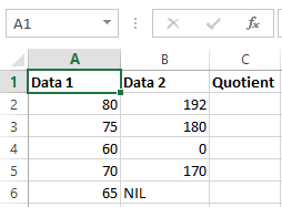
In the table above, we have three columns: Data 1, Data 2, and Quotient.
The idea here is to fill the third column (Quotient) with the result gotten from dividing Data 1 by Data 2.
That is:
For row one: 80/192
For row two: 75/180. And so on.
But if you look closely, some rows have values that will lead to mathematical errors — row 4 and row 6.
We cannot divide 60 by 0 on row 4, nor can we divide 65 by NIL on row 6.
Here's what the table will look like after the divisions:
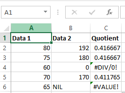
The quotient for column 4 and 6 are #DIV/0! and #VALUE!, respectively. This is because the operation being performed leads to a math error.
We cannot fix this mathematically, but we can catch errors like these and return a custom value for them. Here's how using the IFERROR function:
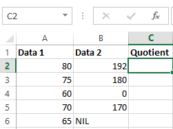
I've removed every value in the Quotient column. Next, we'll use the IFERROR function. That is:
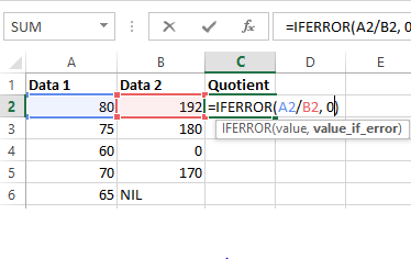
In the first Quotient row, we wrote the IFERROR function: =IFERROR(A2/B2, 0). The two parameters are A2/B2 and 0.
The first parameter A2/B2 denotes A2 (80)divided by row B2 (192). If the division is possible, the quotient will be returned.
If the division is not possible, the second parameter (0) will be returned.
So our table will look like this after the IFERROR function is applied in each row:
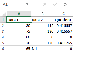
Now row 4 and 6 have 0 as their quotient instead of #DIV/0! and #VALUE!, respectively.
Note that you can use a custom message as well instead of 0. That is: =IFERROR(A2/B2, "Division not possible"). You have to nest the text in quotation marks. We'll have a table like this:
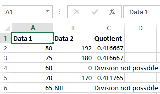
So it's up to you to customize what will be returned if there is an error.
Summary
In this article, we talked about the IFERROR function in Excel. It can be used to handle #N/A, #VALUE!, #REF!, #DIV/0!, #NUM!, #NAME?, or #NULL! errors.
We saw the syntax for using the IFERROR function and the meaning of its parameters.
We also saw some examples that showed how to use the IFERROR function in an Excel table.
Thank you for reading!
ihechikara.com
If you read this far, thank the author to show them you care.
Learn to code for free. freeCodeCamp's open source curriculum has helped more than 40,000 people get jobs as developers. Get started
Recommend
About Joyk
Aggregate valuable and interesting links.
Joyk means Joy of geeK