I recently showed how to compute a bootstrap percentile confidence interval in SAS. The percentile interval is a simple "first-order" interval that is formed from quantiles of the bootstrap distribution. However, it has two limitations. First, it does not use the estimate for the original data; it is based only on bootstrap resamples. Second, it does not adjust for skewness in the bootstrap distribution. The so-called bias-corrected and accelerated bootstrap interval (the BCa interval) is a second-order accurate interval that addresses these issues. This article shows how to compute the BCa bootstrap interval in SAS. You can download the complete SAS program that implements the BCa computation.

As in the previous article, let's bootstrap the skewness statistic for the petal widths of 50 randomly selected flowers of the species Iris setosa. The following statements create a data set called SAMPLE and the rename the variable to analyze to 'X', which is analyzed by the rest of the program:

data sample;
   set sashelp.Iris;     /* <== load your data here */
   where species = "Setosa";
   rename PetalWidth=x;  /* <== rename the analyzes variable to 'x' */
run;

BCa interval: The main ideas

The main advantage to the BCa interval is that it corrects for bias and skewness in the distribution of bootstrap estimates. The BCa interval requires that you estimate two parameters. The bias-correction parameter, z0, is related to the proportion of bootstrap estimates that are less than the observed statistic. The acceleration parameter, a, is proportional to the skewness of the bootstrap distribution. You can use the jackknife method to estimate the acceleration parameter.

Assume that the data are independent and identically distributed. Suppose that you have already computed the original statistic and a large number of bootstrap estimates, as shown in the previous article. To compute a BCa confidence interval, you estimate z0 and a and use them to adjust the endpoints of the percentile confidence interval (CI). If the bootstrap distribution is positively skewed, the CI is adjusted to the right. If the bootstrap distribution is negatively skewed, the CI is adjusted to the left.

Estimate the bias correction and acceleration

The mathematical details of the BCa adjustment are provided in Chernick and LaBudde (2011) and Davison and Hinkley (1997). My computations were inspired by Appendix D of Martinez and Martinez (2001). To make the presentation simpler, the program analyzes only univariate data.

The bias correction factor is related to the proportion of bootstrap estimates that are less than the observed statistic. The acceleration parameter is proportional to the skewness of the bootstrap distribution. You can use the jackknife method to estimate the acceleration parameter. The following SAS/IML modules encapsulate the necessary computations. As described in the jackknife article, the function 'JackSampMat' returns a matrix whose columns contain the jackknife samples and the function 'EvalStat' evaluates the statistic on each column of a matrix.

proc iml;
load module=(JackSampMat);             /* load helper function */
 
/* compute bias-correction factor from the proportion of bootstrap estimates 
   that are less than the observed estimate 
*/
start bootBC(bootEst, Est);
   B = ncol(bootEst)*nrow(bootEst);    /* number of bootstrap samples */
   propLess = sum(bootEst < Est)/B;    /* proportion of replicates less than observed stat */
   z0 = quantile("normal", propLess);  /* bias correction */
   return z0;
finish;
 
/* compute acceleration factor, which is related to the skewness of bootstrap estimates.
   Use jackknife replicates to estimate.
*/
start bootAccel(x);
   M = JackSampMat(x);                 /* each column is jackknife sample */
   jStat = EvalStat(M);                /* row vector of jackknife replicates */
   jackEst = mean(jStat`);             /* jackknife estimate */
   num = sum( (jackEst-jStat)##3 );
   den = sum( (jackEst-jStat)##2 );
   ahat = num / (6*den##(3/2));        /* ahat based on jackknife ==> not random */
   return ahat;
finish;

Compute the BCa confidence interval

With those helper functions defined, you can compute the BCa confidence interval. The following SAS/IML statements read the data, generate the bootstrap samples, compute the bootstrap distribution of estimates, and compute the 95% BCa confidence interval:

/* Input: matrix where each column of X is a bootstrap sample. 
   Return a row vector of statistics, one for each column. */
start EvalStat(M); 
   return skewness(M);               /* <== put your computation here */
finish;
 
alpha = 0.05;
B = 5000;                            /* B = number of bootstrap samples */
use sample; read all var "x"; close; /* read univariate data into x */
 
call randseed(1234567);
Est = EvalStat(x);                   /* 1. compute observed statistic */
s = sample(x, B // nrow(x));         /* 2. generate many bootstrap samples (N x B matrix) */
bStat = T( EvalStat(s) );            /* 3. compute the statistic for each bootstrap sample */
bootEst = mean(bStat);               /* 4. summarize bootstrap distrib, such as mean */
z0 = bootBC(bStat, Est);             /* 5. bias-correction factor */
ahat = bootAccel(x);                 /* 6. ahat = acceleration of std error */
print z0 ahat;
 
/* 7. adjust quantiles for 100*(1-alpha)% bootstrap BCa interval */
zL = z0 + quantile("normal", alpha/2);    
alpha1 = cdf("normal", z0 + zL / (1-ahat*zL));
zU = z0 + quantile("normal", 1-alpha/2);
alpha2 = cdf("normal", z0 + zU / (1-ahat*zU));
call qntl(CI, bStat, alpha1//alpha2); /* BCa interval */
 
R = Est || BootEst || CI`;          /* combine results for printing */
print R[c={"Obs" "BootEst" "LowerCL" "UpperCL"} format=8.4 L="95% Bootstrap Bias-Corrected CI (BCa)"];

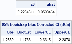
The BCa interval is [0.66, 2.29]. For comparison, the bootstrap percentile CI for the bootstrap distribution, which was computed in the previous bootstrap article, is [0.49, 1.96].

Notice that by using the bootBC and bootAccel helper functions, the program is compact and easy to read. One of the advantages of the SAS/IML language is the ease with which you can define user-defined functions that encapsulate sub-computations.

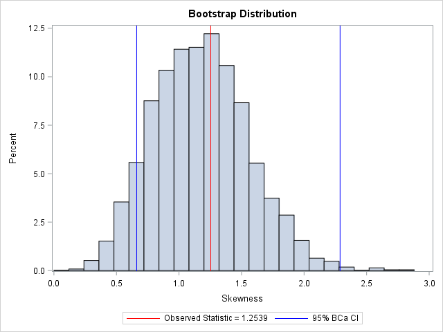
You can visualize the analysis by plotting the bootstrap distribution overlaid with the observed statistic and the 95% BCa confidence interval. Notice that the BCa interval is not symmetric about the bootstrap estimate. Compared to the bootstrap percentile interval (see the previous article), the BCa interval is shifted to the right.

There is another second-order method that is related to the BCa interval. It is called the ABC method and it uses an analytical expression to approximate the endpoints of the BCa interval. See p. 214 of Davison and Hinkley (1997).

In summary, bootstrap computations in the SAS/IML language can be very compact. By writing and re-using helper functions, you can encapsulate some of the tedious calculations into a high-level function, which makes the resulting program easier to read. For univariate data, you can often implement bootstrap computations without writing any loops by using the matrix-vector nature of the SAS/IML language.

If you do not have access to SAS/IML software or if the statistic that you want to bootstrap is produced by a SAS procedure, you can use SAS-supplied macros (%BOOT, %JACK,...) for bootstrapping. The macros include the %BOOTCI macro, which supports the percentile interval, the BCa interval, and others. For further reading, the web page for the macros includes a comparison of the CI methods.