Kernel Ridge Regression Using C#

The Data Science Lab

Kernel Ridge Regression Using C#

KRR is especially useful when there is limited training data, says Dr. James McCaffrey of Microsoft Research in this full-code, step-by-step tutorial.

• By James McCaffrey
• 08/15/2023

• Get Code Download

The goal of a machine learning regression problem is to predict a single numeric value. For example, you might want to predict a person's annual income based on their age, number years of schooling, high school grade point average and so on.

There are roughly a dozen major regression techniques, and each technique has several variations. Among the most common techniques are linear regression, linear ridge regression, k-nearest neighbors regression, kernel ridge regression, Gaussian process regression, decision tree regression and neural network regression. Each technique has pros and cons. This article explains how to implement kernel ridge regression from scratch, using the C# language.

Kernel ridge regression (KRR) is a technique that uses what is called the kernel trick (the "kernel" in KRR) to deal with complex non-linear data, and L2 regularization (the "ridge" in KRR) to avoid model overfitting where a model predicts training data well but predicts new, previously unseen data poorly. KRR is especially useful when there is limited training data.

A good way to see where this article is headed is to take a look at the screenshot of a demo program in Figure 1. The demo program uses synthetic data that was generated by a 5-10-1 neural network with random weights. There are five predictor variables which have values between -1.0 and +1.0, and a target variable to predict which is a value between 0.0 and 1.0. There are 40 training items and 10 test items.

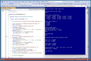
The demo program creates a kernel ridge regression model using the training data. The model uses two parameters. A gamma parameter is set to 0.1 and is used by the model's internal radial basis function (RBF), which is a key component of a KRR model. An alpha parameter is set to 0.001 and is used by the L2 regularization component. The values of gamma and alpha can be determined by trial and error, either manually or programmatically.

After the KRR model is created, it is applied to the training and test data. The model scores 100 percent accuracy on the training data (40 out of 40 correct) and 80 percent accuracy on the test data (8 out of 10 correct). A correct prediction is one that is within 10 percent of the true target value.

The demo program computes and displays the root mean squared error (RMSE) of the model. RMSE is a more granular metric than accuracy but RMSE is more difficult to interpret. The RMSE on the training data is 0.0030 and 0.0308 on the test data. Because the RMSE on the training data is significantly smaller than the RMSE on the test data, the KRR model is slightly overfitted.

The demo program concludes by making a prediction for a new, previously unseen data item x = (0.5, -0.5, 0.5, -0.5, 0.5). The predicted y value is 0.0878.

This article assumes you have intermediate or better programming skill but doesn't assume you know anything about kernel ridge regression. The demo is implemented using C#, but you should be able to refactor the code to a different C-family language if you wish.

The source code for the demo program is too long to be presented in its entirety in this article. The complete code is available in the accompanying file download. The demo code and data are also available online.

Understanding Kernel Ridge Regression
Kernel ridge regression is probably best explained by using a concrete example. The key idea in KRR is a kernel function. A kernel function accepts two vectors and returns a number which is a measure of their similarity. There are many different kernel functions, and there are several variations of each type of kernel function. The most commonly used kernel function (in the projects I've been involved with at any rate) is the radial basis function (RBF).

The form of the RBF function used by the demo program is rbf(x1, x2) = exp( -gamma * ||x1 - x2|| ) where x1 and x2 are two vectors, ||x1 - x2|| is the squared Euclidean distance between x1 and x2, and gamma is a constant.

Suppose x1 = (0.1, 0.5, 0.2) and x2 = (0.4, 0.3, 0.0) and gamma = +1.0. The squared Euclidean distance, ||x1 - x2||, is the sum of the squared differences of the vector elements: (0.1 - 0.4)^2 + (0.5 - 0.3)^2 + (0.2 - 0.0)^2 = 0.09 + 0.04 + 0.04 = 0.17. Therefore, rbf(x1, x2) = exp( -1.0 * 0.17) = exp(-0.17) = 0.8437.

If two vectors are identical (maximum similarity), their RBF is 1.0. As the two vectors decrease in similarity, the RBF value approaches, but never quite reaches, 0.0.

The demo program uses this particular version of RBF because it's the version used by the scikit-learn code library KernelRidge module. Another common version of RBF is rbf(x1, x2) = exp( -1 * ||x1 - x2|| / (2 * s^2) ) where s is a constant called the length scale.

Now suppose that you have just four training data items, where each item has three predictor values:

   X                     y
x0 = [0.1, 0.5, 0.2]  y0 = 0.3
x1 = [0.4, 0.3, 0.0]  y1 = 0.9
x2 = [0.6, 0.1, 0.8]  y2 = 0.4
x3 = [0.0, 0.2, 0.7]  y3 = 0.9

Training a KRR model produces one weight per training item. The weights are sometimes called the dual coefficients. Suppose the four weights are computed to be (w0, w1, w2, w3) = (-3.7, 3.3, -1.2, 2.5). The predicted y for a new x is the sum of the weights times the kernel function applied to x and each training vector. Suppose x = (0.5, 0.4, 0.6) and RBF gamma is set to 1.0, then (subject to rounding):

y_pred = w0 * rbf(x, x0) +
         w1 * rbf(x, x1) +
         w2 * rbf(x, x2) +
         w3 * rbf(x, x3)

       = -3.7 * rbf(x, x0) +
          3.3 * rbf(x, x1) +
         -1.2 * rbf(x, x2) +
          2.5 * rbf(x, x3)

       = -3.7 * 0.72 +
          3.3 * 0.69 +
         -1.2 * 0.87 +
          2.5 * 0.74
   
       = -2.6 + 2.2 + -1.0 + 1.8 
       =  0.40

OK, but where do the weight values come from? Expressed mathematically:

(1) w * K(X', X') = Y'
(2) w * K(X', X') * inv(K(X', X')) = Y' * inv(K(X', X'))
(3) w = Y' * inv(K(X', X'))
(4) y = w * K(X, X')

The w is the vector of the weights. X' is a matrix of training X values. Y' is a vector of training target y values. K(X', X') is a kernel matrix that consists of all possible pairs of RBF values applied to pairs of training X values. The * indicates matrix multiplication and inv() indicates matrix inversion.

Equation (1) is the starting assumption. In equation (2) both sides have been post-matrix-multiplied by inv(K(X', X')). Because A * inv(A) = I (identity), the result simplifies to equation (3). In words, to calculate the model prediction weights, compute the kernel matrix of all pairs of training X data, then find the inverse of that matrix, then multiply by the target Y values. Equation (4) shows how to predict a y value from inputs X by multiplying the weights found in (3) by the kernel matrix of X and all training predictors X'.

The discussion so far explains the "kernel" part of KRR. The L2 regularization "ridge" part is implemented by adding a small alpha value to the diagonal of the kernel matrix, just before applying the matrix inverse operation. In addition to supplying regularization, adding alpha to the K matrix has a nice side effect. If two or more columns of a matrix are mathematically correlated -- for example, the values in column 2 are all exactly three times the values in column 1 -- then matrix inversion will fail. Adding alpha to the K matrix diagonal conditions the matrix and prevents this from happening.

Because KRR adds the same small constant alpha value to each column of the K(X', X') matrix, the predictor data should be normalized to roughly the same scale. The three most common normalization techniques are divide-by-k, min-max and z-score. I recommend divide-by k. For example, if one of the predictor variables is a person's age, you could divide all ages by 100 so that the normalized values are all between 0.0 and 1.0.

Overall Program Structure
I used Visual Studio 2022 (Community Free Edition) for the demo program. I created a new C# console application and checked the "Place solution and project in the same directory" option. I specified .NET version 6.0. I named the project KernelRidgeRegression. I checked the "Do not use top-level statements" option to avoid the confusing program entry point shortcut syntax.

The demo has no significant .NET dependencies and any relatively recent version of Visual Studio with .NET (Core) or the older .NET Framework will work fine. You can also use the Visual Studio Code program if you like.

After the template code loaded into the editor, I right-clicked on file Program.cs in the Solution Explorer window and renamed the file to the more descriptive KernelRidgeRegressionProgram.cs. I allowed Visual Studio to automatically rename class Program.

The overall program structure is presented in Listing 1. The Program class houses the Main() method and helper Accuracy() and RootMSE() functions. The KRR class houses all the kernel ridge regression functionality such as the Train() and Predict() methods. The Utils class houses all the matrix helper functions such as MatLoad() to load data into a matrix from a text file, and MatInverse() to find the inverse of a matrix.

Listing 1: Overall Program Structure

using System;
using System.IO;

namespace KernelRidgeRegression
{
  internal class KernelRidgeRegressionProgram
  {
    static void Main(string[] args)
    {
      Console.WriteLine("Begin C# KRR ");

      // 1. load train and test data into memory
      // 2. create and train KRR model
      // 3. evaluate KRR model
      // 4. use model to make a prediction

      Console.WriteLine("End KRR demo ");
      Console.ReadLine();
    } // Main()

    static double Accuracy(KRR model, 
      double[][] dataX, double[] dataY,
      double pctClose) { . . }
    
    static double RootMSE(KRR model,
      double[][] dataX, double[] dataY) { . . }
    
  } // class Program

  public class KRR
  {
    public double gamma;  // for RBF kernel
    public double alpha;  // regularization
    public double[][] trainX;  // need for prediction
    public double[] wts;  // one per trainX item

    public KRR(double gamma, double alpha)
    {
      this.gamma = gamma;
      this.alpha = alpha;
    } // ctor

    public void Train(double[][] trainX,
      double[] trainY) { . . }
    
    public double Rbf(double[] v1,
      double[] v2) { . . }
    
    public double Predict(double[] x) { . . }
  } // class KRR

  public class Utils
  {
    public static double[][] MatCreate(int rows,
      int cols) { . . }
    
    public static double[] MatToVec(double[][] m)
      { . . }
    
    public static double[][] MatProduct(double[][]
      matA, double[][] matB) { . . }
    
    public static double[][] VecToMat(double[] vec,
      int nRows, int nCols) { . . }
    
    public static double[] VecMatProd(double[] v,
      double[][] m) { . . }
    
    public static double[][] MatTranspose(double[][]
      m) { . . }
    
    public static double[][] MatInverse(double[][]
      m) { . . }
    
    static int MatDecompose(double[][] m,
      out double[][] lum, out int[] perm) { . . }
    
    static double[] Reduce(double[][] luMatrix,
      double[] b) { . . }
    
    static int NumNonCommentLines(string fn,
      string comment) { . . }
    
    public static double[][] MatLoad(string fn,
      int[] usecols, char sep, string comment) { . . }
    
    public static void MatShow(double[][] m,
      int dec, int wid) { . . }
    
    public static void VecShow(double[] vec,
      int dec, int wid, bool newLine) { . . }
    
  } // class Utils
} // ns

Although the demo program is long, over 60 percent of the code is in the helper Utils class. The demo program begins by loading the synthetic training data into memory:

Console.WriteLine("Loading train and test data ");
string trainFile =
  "..\\..\\..\\Data\\synthetic_train.txt";
double[][] trainX =
  Utils.MatLoad(trainFile,
  new int[] { 0, 1, 2, 3, 4 }, '\t', "#");  // 40 items
double[] trainY =
  Utils.MatToVec(Utils.MatLoad(trainFile,
  new int[] { 5 }, '\t', "#"));

The code assumes the data is located in a subdirectory named Data. The MatLoad() utility function specifies that the data is tab delimited and uses the '#' character to identify lines that are comments. The test data is loaded into memory in the same way:

string testFile =
  "..\\..\\..\\Data\\synthetic_test.txt";
double[][] testX =
  Utils.MatLoad(testFile,
  new int[] { 0, 1, 2, 3, 4 }, '\t', "#");  // 10 items
double[] testY =
  Utils.MatToVec(Utils.MatLoad(testFile,
  new int[] { 5 }, '\t', "#"));
Console.WriteLine("Done ");

Next, the demo displays the first three test predictor values and target values:

Console.WriteLine("First three X predictors: ");
for (int i = 0; i < 3; ++i)
  Utils.VecShow(trainX[i], 4, 9, true);
Console.WriteLine("First three target y: ");
for (int i = 0; i < 3; ++i)
  Console.WriteLine(trainY[i].
  ToString("F4").PadLeft(8));

In a non-demo scenario you'd probably want to display all training and test data to make sure it was loaded correctly. The kernel ridge regression model is created using the class constructor:

Console.WriteLine("Creating KRR object");
double gamma = 0.1;    // RBF param
double alpha = 0.001;  // regularization
Console.WriteLine("Setting RBF gamma = " +
  gamma.ToString("F1"));
Console.WriteLine("Setting alpha noise =  " +
  alpha.ToString("F3"));
KRR krr = new KRR(gamma, alpha);
Console.WriteLine("Done ");

The KRR constructor accepts values for the gamma and alpha parameters. These values must be determined by experimentation. Larger values of alpha retard the magnitudes of the model coefficients, which improves generalizability, but at the expense of accuracy.