

A First course in FEM —— matlab代码实现求解传热问题(稳态) - blogzzt
source link: https://www.cnblogs.com/spacerunnerZ/p/17488576.html
Go to the source link to view the article. You can view the picture content, updated content and better typesetting reading experience. If the link is broken, please click the button below to view the snapshot at that time.

这篇文章会将FEM全流程走一遍,包括网格、矩阵组装、求解、后处理。内容是大三时的大作业,今天拿出来回顾下。
1. 问题简介
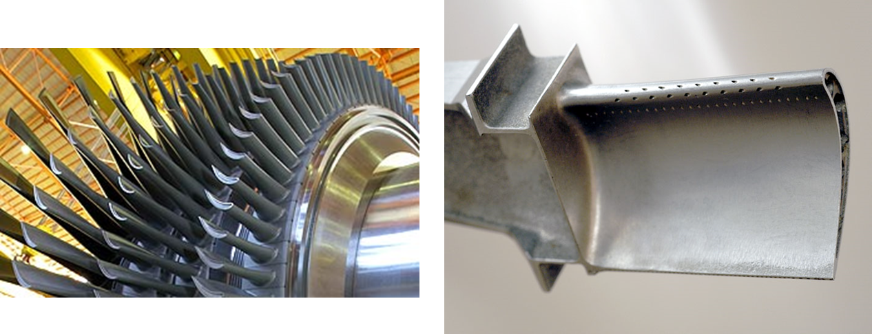
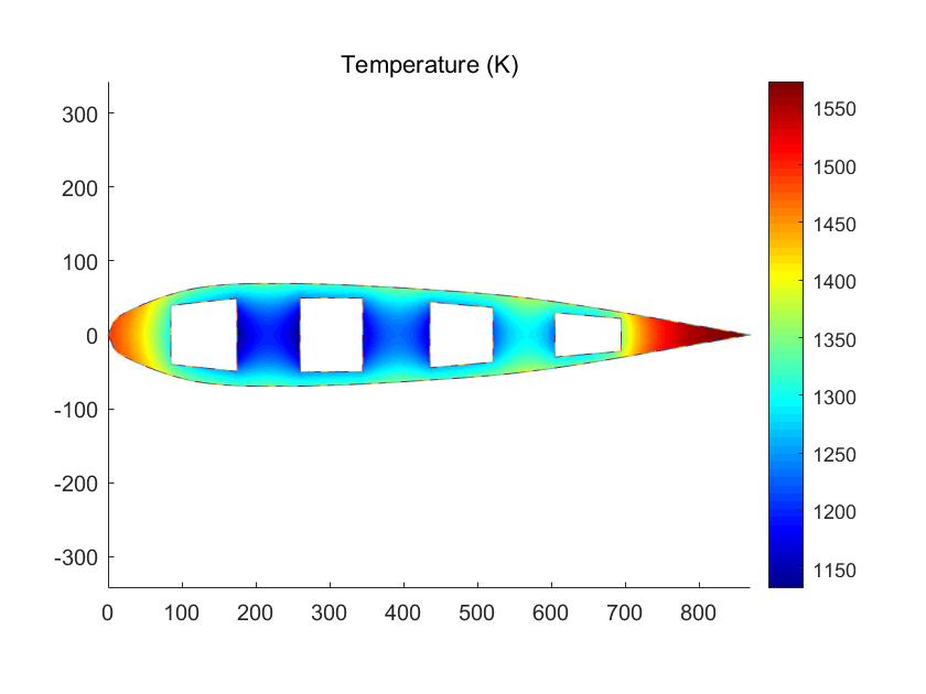
涡轮机叶片需要冷却以提高涡轮的性能和涡轮叶片的寿命。我们现在考虑一个如上图所示的叶片,叶片处在一个高温环境中,中间通有四个冷却孔。
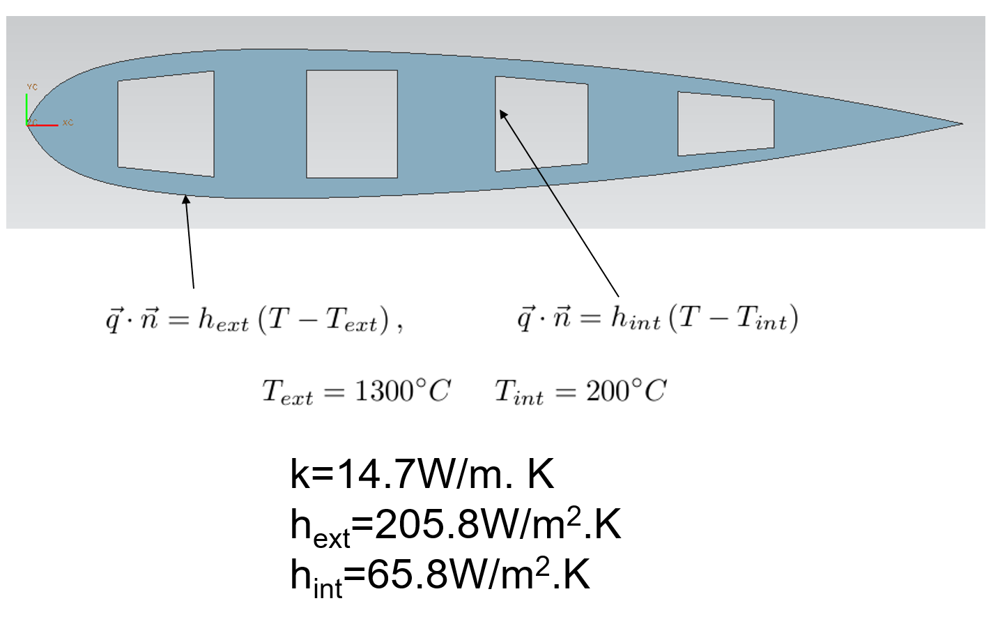
假设为稳态,那么叶片内导热微分方程为:
内部区域: ![]() (扩散方程)
(扩散方程)
![]() (外表面)
(外表面)
![]() (内部冷却孔)
(内部冷却孔)
2.1几何模型
我们简化为二维模型,如下图所示:
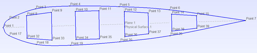
1:0.0,0.0 6:597.6,45.9 11:344.7,50.0
2:20.9,28.8 7:870.0,0.0 12:435.8,44.5
3:117.4,62.9 8:85.0,40.0 13:521.2,37.0
4:240.4,69.6 9:174.5,49.4 14:605.0,30.0
5:417.5,62.4 10:260.0,50.0 15:694.7,22.2
2.2 单位系统和物性
长度单位:mm
温度单位: K
功率单位:W
k=14.7*10^-3 W/mm. K
hext=205.8*10^-6 W/m2.K
hint=65.8*10^-6 W/m2.K
注意:在后面的矩阵组装中的h_wall = h / k
2.3网格
用开源软件Gmsh生成网格。
首先写geo文件
注意要把外表面和中间空洞用Physical Line定义
lc = 10;
Point(1) = {0, 0, 0, lc};
Point(2) = {20.9,28.8,0, lc};
Point(3) = {117.4,62.9,0, lc};
Point(4) = {240.4,69.6,0, lc};
Point(5) =  {417.5,62.4,0, lc};
Point(6) = {597.6,45.9,0, lc};
Point(7) = {870.0,0.0, 0,lc};
Point(8) = {85.0,40.0, 0,lc};
Point(9) = {174.5,49.4,0, lc};
Point(10) = {260.0,50.0,0, lc};
Point(11) = {344.7,50.0,0, lc};
Point(12) = {435.8,44.5,0, lc};
Point(13) = {521.2,37.0,0, lc};
Point(14) = {605.0,30.0,0, lc};
Point(15) = {694.7,22.2,0, lc};

//+
Spline(1) = {1, 2, 3, 4, 5, 6, 7};
//+
Symmetry {0, 1, 0, 0} {
  Duplicata { Point{1}; Point{2}; Point{3}; Point{4}; Point{5}; Line{1}; Point{6}; Point{7}; Point{8}; Point{9}; Point{10}; Point{11}; Point{12}; Point{13}; Point{14}; Point{15}; }
}

//+
Line Loop(1) = {1, -2};
//+
Line(3) = {8, 9};
//+
Line(4) = {9, 33};
//+
Line(5) = {33, 32};
//+
Line(6) = {32, 8};
//+
Line(7) = {10, 11};
//+
Line(8) = {11, 35};
//+
Line(9) = {35, 34};
//+
Line(10) = {34, 10};
//+
Line(11) = {12, 13};
//+
Line(12) = {13, 37};
//+
Line(13) = {37, 36};
//+
Line(14) = {36, 12};
//+
Line(15) = {14, 15};
//+
Line(16) = {15, 39};
//+
Line(17) = {39, 38};
//+
Line(18) = {38, 14};
//+
Line Loop(2) = {3, 4, 5, 6};
//+
Line Loop(3) = {7, 8, 9, 10};
//+
Line Loop(4) = {11, 12, 13, 14};
//+
Line Loop(5) = {15, 16, 17, 18};
//+
Physical Line(0)={1, -2};
Physical Line(1)={3, 4, 5, 6};
Physical Line(2)={7, 8, 9, 10};
Physical Line(3)={11, 12, 13, 14};
Physical Line(4)={15, 16, 17, 18};

Plane Surface(1) = {1, 2, 3, 4, 5};
Physical Surface(1) = {1};
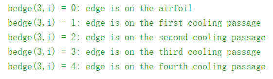
边界信息如何保存?
边界edges需要用标记,
在matlab程序中用bedge(3,Nbc)存储边界信息,前两个数字代表边的两端节点编号,第三个数字代表属于哪一个边。

生成网格后导出为“blademesh.m”用以后续使用,注意不要勾选Save all elements,否则会没有边界信息。
我用gmsh-4.4.1-Windows64版本,可以导出边界信息。但是新版的gmsh导出为.m文件时,边界信息无法保存。

3. 矩阵组装
3.1 控制方程
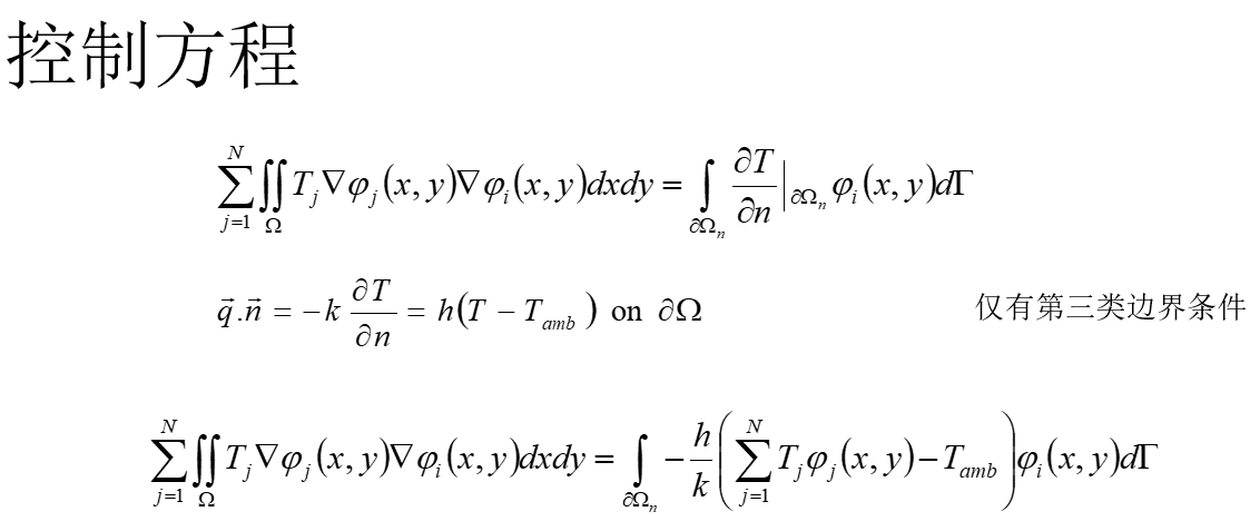
3.2 系统矩阵

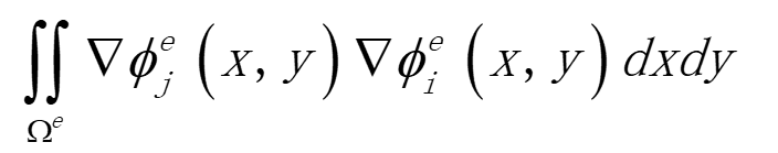
其中的Ω代表全域,我们将全域分解为一个个单元,这就是有限元的思想。
计算每个单元(Ωe)的刚度矩阵,然后每项加到整体刚度矩阵:
4. 代码实现(matlab)
|
步骤 |
工具或函数 |
|
定义求解域并生成网格 |
gmsh导出网格为blademesh.m |
|
读入网格信息,数据转换 |
bladeread |
|
矩阵和矢量组装,线性方程组求解 |
bleadheat |
|
bladeplot |
主程序:bladeheat.m
% Clear variables

clear all;


% Set gas temperature and wall heat transfer coefficients at
% boundaries of the blade.  Note: Tcool(i) and hwall(i) are the
% values of Tcool and hwall for the ith boundary which are numbered
% as follows:
%
%   1 = external boundary (airfoil surface)
%   2 = 1st internal cooling passage (from leading edge)
%   3 = 2nd internal cooling passage (from leading edge)
%   3 = 3rd internal cooling passage (from leading edge)
%   3 = 4th internal cooling passage (from leading edge)

% Tcool = [1300, 200, 200, 200, 200];
% hwall = [14, 4.7, 4.7, 4.7, 4.7];

Tcool = [1573, 473, 473, 473, 473];
h = [205.8*10^-6, 65.8*10^-6, 65.8*10^-6, 65.8*10^-6, 65.8*10^-6];
k = 14.7*10^-3;
hwall = h / k;


% Load in the grid file
% NOTE:  after loading a gridfile using the load(fname) command,
%        three important grid variables and data arrays exist.  These are:
%
% Nt: Number of triangles (i.e. elements) in mesh
%
% Nv: Number of nodes (i.e. vertices) in mesh
%
% Nbc: Number of edges which lie on a boundary of the computational
%      domain.
%
% tri2nod(3,Nt):  list of the 3 node numbers which form the current
%                 triangle.  Thus, tri2nod(1,i) is the 1st node of
%                 the i'th triangle, tri2nod(2,i) is the 2nd node
%                 of the i'th triangle, etc.
%
% xy(2,Nv): list of the x and y locations of each node.  Thus,
%           xy(1,i) is the x-location of the i'th node, xy(2,i)
%           is the y-location of the i'th node, etc.
%
% bedge(3,Nbc): For each boundary edge, bedge(1,i) and bedge(2,i)
%               are the node numbers for the nodes at the end
%               points of the i'th boundary edge.  bedge(3,i) is an
%               integer which identifies which boundary the edge is
%               on. In this solver, the third value has the
%               following meaning:
%
%               bedge(3,i) = 0: edge is on the airfoil
%               bedge(3,i) = 1: edge is on the first cooling passage
%               bedge(3,i) = 2: edge is on the second cooling passage
%               bedge(3,i) = 3: edge is on the third cooling passage
%               bedge(3,i) = 4: edge is on the fourth cooling passage
%
bladeread;

% Start timer
Time0 = cputime;

% Zero stiffness matrix

K = zeros(Nv, Nv);
b = zeros(Nv, 1);

% Zero maximum element size
hmax = 0;

% Loop over elements and calculate residual and stiffness matrix

for ii = 1:Nt,

  kn(1) = tri2nod(1,ii);
  kn(2) = tri2nod(2,ii);
  kn(3) = tri2nod(3,ii);

  xe(1) = xy(1,kn(1));
  xe(2) = xy(1,kn(2));
  xe(3) = xy(1,kn(3));

  ye(1) = xy(2,kn(1));
  ye(2) = xy(2,kn(2));
  ye(3) = xy(2,kn(3));

  % Calculate circumcircle radius for the element
  % First, find the center of the circle by intersecting the median
  % segments from two of the triangle edges.

  dx21 = xe(2) - xe(1);
  dy21 = ye(2) - ye(1);

  dx31 = xe(3) - xe(1);
  dy31 = ye(3) - ye(1);

  x21  = 0.5*(xe(2) + xe(1));
  y21  = 0.5*(ye(2) + ye(1));

  x31  = 0.5*(xe(3) + xe(1));
  y31  = 0.5*(ye(3) + ye(1));

  b21 = x21*dx21 + y21*dy21;
  b31 = x31*dx31 + y31*dy31;

  xydet = dx21*dy31 - dy21*dx31;

  x0 = (dy31*b21 - dy21*b31)/xydet;
  y0 = (dx21*b31 - dx31*b21)/xydet;

  Rlocal = sqrt((xe(1)-x0)^2 + (ye(1)-y0)^2);

  if (hmax < Rlocal),
    hmax = Rlocal;
  end

  % Calculate all of the necessary shape function derivatives, the
  % Jacobian of the element, etc.

  % Derivatives of node 1's interpolant
  dNdxi(1,1) = -1.0; % with respect to xi1
  dNdxi(1,2) = -1.0; % with respect to xi2

  % Derivatives of node 2's interpolant
  dNdxi(2,1) =  1.0; % with respect to xi1
  dNdxi(2,2) =  0.0; % with respect to xi2

  % Derivatives of node 3's interpolant
  dNdxi(3,1) =  0.0; % with respect to xi1
  dNdxi(3,2) =  1.0; % with respect to xi2

  % Sum these to find dxdxi (note: these are constant within an element)
  dxdxi = zeros(2,2);
  for nn = 1:3,
    dxdxi(1,:) = dxdxi(1,:) + xe(nn)*dNdxi(nn,:);
    dxdxi(2,:) = dxdxi(2,:) + ye(nn)*dNdxi(nn,:);
  end

  % Calculate determinant for area weighting
  J = dxdxi(1,1)*dxdxi(2,2) - dxdxi(1,2)*dxdxi(2,1);
  A = 0.5*abs(J); % Area is half of the Jacobian

  % Invert dxdxi to find dxidx using inversion rule for a 2x2 matrix
  dxidx = [ dxdxi(2,2)/J, -dxdxi(1,2)/J; ...
       -dxdxi(2,1)/J,  dxdxi(1,1)/J];

  % Calculate dNdx
  dNdx = dNdxi*dxidx;

  % Add contributions to stiffness matrix for node 1 weighted residual
  K(kn(1), kn(1)) = K(kn(1), kn(1)) + (dNdx(1,1)*dNdx(1,1) + dNdx(1,2)*dNdx(1,2))*A;
  K(kn(1), kn(2)) = K(kn(1), kn(2)) + (dNdx(1,1)*dNdx(2,1) + dNdx(1,2)*dNdx(2,2))*A;
  K(kn(1), kn(3)) = K(kn(1), kn(3)) + (dNdx(1,1)*dNdx(3,1) + dNdx(1,2)*dNdx(3,2))*A;

  % Add contributions to stiffness matrix for node 2 weighted residual
  K(kn(2), kn(1)) = K(kn(2), kn(1)) + (dNdx(2,1)*dNdx(1,1) + dNdx(2,2)*dNdx(1,2))*A;
  K(kn(2), kn(2)) = K(kn(2), kn(2)) + (dNdx(2,1)*dNdx(2,1) + dNdx(2,2)*dNdx(2,2))*A;
  K(kn(2), kn(3)) = K(kn(2), kn(3)) + (dNdx(2,1)*dNdx(3,1) + dNdx(2,2)*dNdx(3,2))*A;

  % Add contributions to stiffness matrix for node 3 weighted residual
  K(kn(3), kn(1)) = K(kn(3), kn(1)) + (dNdx(3,1)*dNdx(1,1) + dNdx(3,2)*dNdx(1,2))*A;
  K(kn(3), kn(2)) = K(kn(3), kn(2)) + (dNdx(3,1)*dNdx(2,1) + dNdx(3,2)*dNdx(2,2))*A;
  K(kn(3), kn(3)) = K(kn(3), kn(3)) + (dNdx(3,1)*dNdx(3,1) + dNdx(3,2)*dNdx(3,2))*A;

end


% Loop over boundary edges and account for bc's
% Note: the bc's are all convective heat transfer coefficient bc's
% so the are of 'Robin' form.  This requires modification of the
% stiffness matrix as well as impacting the right-hand side, b.
%

for ii = 1:Nbc,

  % Get node numbers on edge
  kn(1) = bedge(1,ii);
  kn(2) = bedge(2,ii);

  % Get node coordinates
  xe(1) = xy(1,kn(1));
  xe(2) = xy(1,kn(2));

  ye(1) = xy(2,kn(1));
  ye(2) = xy(2,kn(2));

  % Calculate edge length
  ds = sqrt((xe(1)-xe(2))^2 + (ye(1)-ye(2))^2);

  % Determine the boundary number
  bnum = bedge(3,ii) + 1;

  % Based on boundary number, set heat transfer bc
  K(kn(1), kn(1)) = K(kn(1), kn(1)) + hwall(bnum)*ds*(1/3);
  K(kn(1), kn(2)) = K(kn(1), kn(2)) + hwall(bnum)*ds*(1/6);
  b(kn(1))        = b(kn(1))        + hwall(bnum)*ds*0.5*Tcool(bnum);

  K(kn(2), kn(1)) = K(kn(2), kn(1)) + hwall(bnum)*ds*(1/6);
  K(kn(2), kn(2)) = K(kn(2), kn(2)) + hwall(bnum)*ds*(1/3);
  b(kn(2))        = b(kn(2))        + hwall(bnum)*ds*0.5*Tcool(bnum);

end

% Solve for temperature
Tsol = K\b;

% Finish timer
Time1 = cputime;

% Plot solution
bladeplot;

% Report outputs
Tmax = max(Tsol);
Tmin = min(Tsol);

fprintf('Number of nodes      = %i\n',Nv);
fprintf('Number of elements   = %i\n',Nt);
fprintf('Maximum element size = %5.3f\n',hmax);
fprintf('Minimum temperature  = %6.1f\n',Tmin);
fprintf('Maximum temperature  = %6.1f\n',Tmax);
fprintf('CPU Time (secs)      = %f\n',Time1 - Time0);
bladeread.m
% Read three important grid variables and data arrays
% Nt: Number of triangles (i.e. elements) in mesh
% Nv: Number of nodes (i.e. vertices) in mesh
% Nbc: Number of edges which lie on a boundary of the computational
%      domain.
% tri2nod(3,Nt):  list of the 3 node numbers which form the current
%                 triangle.  Thus, tri2nod(1,i) is the 1st node of
%                 the i'th triangle, tri2nod(2,i) is the 2nd node
%                 of the i'th triangle, etc.
% xy(2,Nv): list of the x and y locations of each node.  Thus,
%           xy(1,i) is the x-location of the i'th node, xy(2,i)
%           is the y-location of the i'th node, etc.
% bedge(3,Nbc): For each boundary edge, bedge(1,i) and bedge(2,i)
%               are the node numbers for the nodes at the end
%               points of the i'th boundary edge.  bedge(3,i) is an
%               integer which identifies which boundary the edge is
%               on. In this solver, the third value has the
%               following meaning:
%
%               bedge(3,i) = 0: edge is on the airfoil
%               bedge(3,i) = 1: edge is on the first cooling passage
%               bedge(3,i) = 2: edge is on the second cooling passage
%               bedge(3,i) = 3: edge is on the third cooling passage
%               bedge(3,i) = 4: edge is on the fourth cooling passage
%

clc
run('blademesh.m');
Nv=msh.nbNod;
Nt=size(msh.TRIANGLES,1);
Nbc=size(msh.LINES,1);
for i=1:Nt
    tri2nod(1,i)=msh.TRIANGLES(i,1);
    tri2nod(2,i)=msh.TRIANGLES(i,2);
    tri2nod(3,i)=msh.TRIANGLES(i,3);
end
for i=1:Nv
    xy(1,i)=msh.POS(i,1);
    xy(2,i)=msh.POS(i,2);
end
for i=1:Nbc
    bedge(1,i)=msh.LINES(i,1);
    bedge(2,i)=msh.LINES(i,2);
    bedge(3,i)=msh.LINES(i,3);
end
bladeplot.m
% Plot T in triangles
figure;
for ii = 1:Nt,
  for nn = 1:3,
    xtri(nn,ii) = xy(1,tri2nod(nn,ii));
    ytri(nn,ii) = xy(2,tri2nod(nn,ii));
    Ttri(nn,ii) = Tsol(tri2nod(nn,ii));
  end
end
HT = patch(xtri,ytri,Ttri);
axis('equal');
set(HT,'LineStyle','none');
title('Temperature (K)');
% caxis([298,1573]);
colormap(jet);
HC = colorbar;
hold on; bladeplotgrid; hold off;
5. 计算结果
Recommend
About Joyk
Aggregate valuable and interesting links.
Joyk means Joy of geeK