

Anomaly Detection in Time Series Data
source link: https://www.geeksforgeeks.org/anomaly-detection-in-time-series-data/
Go to the source link to view the article. You can view the picture content, updated content and better typesetting reading experience. If the link is broken, please click the button below to view the snapshot at that time.

Anomaly Detection in Time Series Data
Anomaly detection is the process of identifying data points or patterns in a dataset that deviate significantly from the norm. A time series is a collection of data points gathered over some time. Anomaly detection in time series data may be helpful in various industries, including manufacturing, healthcare, and finance. Anomaly detection in time series data may be accomplished using unsupervised learning approaches like clustering, PCA (Principal Component Analysis), and autoencoders.
What is an Anomaly Detection Algorithm?
Anomaly detection is the process of identifying data points that deviate from the expected patterns in a dataset. Many applications, including fraud detection, intrusion detection, and failure detection, often use anomaly detection techniques. Finding uncommon or very infrequent events that could point to a possible hazard, issue, or opportunity is the aim of anomaly detection.
The autoencoder algorithm is an unsupervised deep learning algorithm that can be used for anomaly detection in time series data. The autoencoder is a neural network that learns to reconstruct its input data By first compressing input data into a lower-dimensional representation and then extending it back to its original dimensions. An autoencoder may be trained on typical time series data to learn a compressed version of the data for anomaly identification. The anomaly score may then be calculated using the reconstruction error between the original and reconstructed data. Anomalies are data points with considerable reconstruction errors.
Time Series Data and Anamoly Detection
In the case of time series data, anomaly detection algorithms are especially important since they help us spot odd patterns in the data that would not be obvious from just looking at the raw data. Anomalies in time series data might appear as abrupt increases or decrease in values, odd patterns, or unexpected seasonality. Time series data is a collection of observations across time.
- Time series data may be used to teach anomaly detection algorithms, such as the autoencoder, how to represent typical patterns. These algorithms can then utilize this representation to find anomalies. The approach can learn a compressed version of the data by training an autoencoder on regular time series data. The anomaly score may then be calculated using the reconstruction error between the original and reconstructed data. Anomalies are data points with considerable reconstruction errors.
- Anomaly detection algorithms may be applied to time series data to find odd patterns that could point to a hazard, issue, or opportunity. For instance, in the context of predictive maintenance, a time series anomaly may point to a prospective equipment failure that may be fixed before it results in a large amount of downtime or safety concerns. Anomalies in time series data may reveal market movements or patterns in financial forecasts that may be capitalized on.
The reason for getting precision, recall, and F1 score of 1.0 is that the “ambient_temperature_system_failure.csv” dataset from the NAB repository contains anomalies. If we had gotten precision, recall, and F1 score of 0.0, then that means the “ambient_temperature_system_failure.csv” dataset from the NAB repository does not contain anomalies.
Importing Libraries and Dataset
Python libraries make it very easy for us to handle the data and perform typical and complex tasks with a single line of code.
- Pandas – This library helps to load the data frame in a 2D array format and has multiple functions to perform analysis tasks in one go.
- Numpy – Numpy arrays are very fast and can perform large computations in a very short time.
- Matplotlib/Seaborn – This library is used to draw visualizations.
- Sklearn – This module contains multiple libraries having pre-implemented functions to perform tasks from data preprocessing to model development and evaluation.
- TensorFlow – This is an open-source library that is used for Machine Learning and Artificial intelligence and provides a range of functions to achieve complex functionalities with single lines of code.
- Python3
import pandas as pdimport tensorflow as tffrom keras.layers import Input, Densefrom keras.models import Modelfrom sklearn.metrics import precision_recall_fscore_supportimport matplotlib.pyplot as plt |
In this step, we import the libraries required for the implementation of the anomaly detection algorithm using an autoencoder. We import pandas for reading and manipulating the dataset, TensorFlow and Keras for building the autoencoder model, and scikit-learn for calculating the precision, recall, and F1 score.
- Python3
data = pd.read_csv('/NAB/master/data/realKnownCause/ambient''_temperature_system_failure.csv')# Exclude datetime columndata_values = data.drop('timestamp',axis=1).values# Convert data to float typedata_values = data_values.astype('float32')# Create new dataframe with converted valuesdata_converted = pd.DataFrame(data_values,columns=data.columns[1:])# Add back datetime columndata_converted.insert(0, 'timestamp',data['timestamp']) |
We load a dataset called “ambient_temperature_system_failure.csv” from the Numenta Anomaly Benchmark (NAB) dataset, which contains time-series data of ambient temperature readings from a system that experienced a failure.
The panda’s library is used to read the CSV file from a remote location on GitHub and store it in a variable called “data”.
- Now, the code drops the “timestamp” column from the “data” variable, since it is not needed for data analysis purposes. The remaining columns are stored in a variable called “data_values”.
- Then, the “data_values” are converted to the “float32” data type to reduce memory usage, and a new pandas DataFrame called “data_converted” is created with the converted data. The columns of “data_converted” are labeled with the original column names from “data”, except for the “timestamp” column that was previously dropped.
- Finally, the code adds the “timestamp” column back to “data_converted” at the beginning using the “insert()” method. The resulting DataFrame “data_converted” has the same data as “data” but without the unnecessary “timestamp” column, and the data is in a format that can be used for analysis and visualization.
- Python3
data_converted = data_converted.dropna() |
We remove any missing or NaN values from the dataset.
Anomaly Detection using Autoencoder
It is a type of neural network that learns to compress and then reconstruct the original data, allowing it to identify anomalies in the data.
- Python3
# Exclude datetime column againdata_tensor = tf.convert_to_tensor(data_converted.drop('timestamp', axis=1).values, dtype=tf.float32)# Define the autoencoder modelinput_dim = data_converted.shape[1] - 1encoding_dim = 10input_layer = Input(shape=(input_dim,))encoder = Dense(encoding_dim, activation='relu')(input_layer)decoder = Dense(input_dim, activation='relu')(encoder)autoencoder = Model(inputs=input_layer, outputs=decoder)# Compile and fit the modelautoencoder.compile(optimizer='adam', loss='mse')autoencoder.fit(data_tensor, data_tensor, epochs=50,batch_size=32, shuffle=True)# Calculate the reconstruction error for each data pointreconstructions = autoencoder.predict(data_tensor)mse = tf.reduce_mean(tf.square(data_tensor - reconstructions),axis=1)anomaly_scores = pd.Series(mse.numpy(), name='anomaly_scores')anomaly_scores.index = data_converted.index |
We define the autoencoder model and fit it to the cleaned data. The autoencoder is used to identify any deviations from the regular patterns in the data that are learned from the data. To reduce the mean squared error between the input and the output, the model is trained. The reconstruction error for each data point is determined using the trained model and is utilized as an anomaly score.
- Python3
threshold = anomaly_scores.quantile(0.99)anomalous = anomaly_scores > thresholdbinary_labels = anomalous.astype(int)precision, recall,\f1_score, _ = precision_recall_fscore_support(binary_labels, anomalous, average='binary') |
Here, we define an anomaly detection threshold and assess the model’s effectiveness using precision, recall, and F1 score. Recall is the ratio of true positives to all real positives, whereas precision is the ratio of genuine positives to all projected positives. The harmonic mean of recall and accuracy is the F1 score.
- Python3
test = data_converted['value'].valuespredictions = anomaly_scores.valuesprint("Precision: ", precision)print("Recall: ", recall)print("F1 Score: ", f1_score) |
Output:
Precision:  1.0
Recall:  1.0
F1 Score:  1.0
Visualizing the Anomaly
Now let’s plot the anomalies which are predicted by the model and get a feel for whether the predictions made are correct or not by plotting the anomalous examples with red marks with the complete data.
- Python3
# Plot the data with anomalies marked in redplt.figure(figsize=(16, 8))plt.plot(data_converted['timestamp'],data_converted['value'])plt.plot(data_converted['timestamp'][anomalous],data_converted['value'][anomalous], 'ro')plt.title('Anomaly Detection')plt.xlabel('Time')plt.ylabel('Value')plt.show() |
Output:
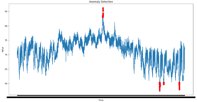
Anomaly represented with red dots on time series data
Recommend
About Joyk
Aggregate valuable and interesting links.
Joyk means Joy of geeK