Time series analysis is a specialized branch of statistics that involves the study of ordered, often temporal data. Its applications span a multitude of fields, including finance, economics, ecology, neuroscience, and physics. Given the temporal dependency of the data, traditional validation techniques such as K-fold cross-validation cannot be applied, thereby necessitating unique methodologies for model training and validation. This comprehensive guide walks you through the crucial aspects of time series analysis, covering topics such as cross-validation techniques, time series decomposition and transformation, feature engineering, derivative utilization, and a broad range of time series modeling techniques. Whether you are a novice just starting out or an experienced data scientist looking to hone your skills, this guide offers valuable insights into the complex yet intriguing world of time series analysis.

Cross-Validation Techniques for Time Series

Executing cross-validation on time series data necessitates adherence to the chronological arrangement of observations. Therefore, traditional methods like K-Fold cross-validation are unsuitable as they jumble the data randomly, disrupting the sequence of time.

Two principal strategies exist for cross-validation on time series data: "Rolling Forecast Origin" and "Expanding Window."

Rolling Forecast Origin Approach

This approach involves a sliding data window for training, followed by a test set right after the training window. With each cycle, the window advances in time, a process also known as "walk-forward" validation.

The Latest DZone Refcard

Getting Started With Distributed SQL

In the following example, the data is segregated into five parts. During each cycle, the model is first trained on the initial part, then on the first and second parts, and so on, testing on the subsequent part each time.

from sklearn.model_selection import TimeSeriesSplit
import numpy as np

# Assuming 'X' and 'y' are your features and target

tscv = TimeSeriesSplit(n_splits=5)

for train_index, test_index in tscv.split(X):
    X_train, X_test = X[train_index], X[test_index]
    y_train, y_test = y[train_index], y[test_index]
    # Fit and evaluate your model here

Expanding Window Technique

The expanding window technique resembles the rolling forecast origin method, but instead of using a fixed-size sliding window, the training set grows over time to incorporate more data.

In this example, we set max_train_size=None to ensure the training set size expands in each iteration. The model is first trained on the first part, then the first and second parts, and so on, testing on the subsequent part each time.

from sklearn.model_selection import TimeSeriesSplit
import numpy as np

# Assuming 'X' and 'y' are your features and target

tscv = TimeSeriesSplit(n_splits=5, max_train_size=None)

for train_index, test_index in tscv.split(X):
    X_train, X_test = X[train_index], X[test_index]
    y_train, y_test = y[train_index], y[test_index]
    # Fit and evaluate your model here

Decomposing and Transforming Time Series

The process of breaking down time series into its constituent parts can significantly aid analysis. This process falls into two categories: decomposing and transforming.

Decomposing of Time Series

Time series dissection is a technique used to break down a time series into its elemental components to facilitate understanding and analysis of underlying patterns and trends. The primary components of a time series are:

Trend: This represents the long-term movement or overall direction of the time series data. It signifies the basic pattern or the general course the data is following.

Seasonality: These are repeating patterns or fluctuations in the time series data that occur at regular intervals, such as daily, weekly, monthly, or yearly. Seasonality is driven by external factors like weather, holidays, or other seasonal events.

Irregular Component: Also termed as noise or residual, this is the unexplained variation in the time series data after removing the trend, seasonality, and cyclical components. It represents random, unpredictable fluctuations that cannot be attributed to any systematic pattern.

In Python, Decomposition can be performed using thestatsmodels or statsforecast libraries:

from statsforecast import StatsForecast
from statsforecast.models import MSTL, AutoARIMA

models = [
    MSTL(
        season_length=[12 * 7],  # seasonalities of the time series
        trend_forecaster=AutoARIMA(),  # model used to forecast trend
    )
]

sf = StatsForecast(
    models=models,  # model used to fit each time series
    freq="D",  # frequency of the data
)
sf = sf.fit(data)
test = sf.fitted_[0, 0].model_
fig, ax = plt.subplots(1, 1, figsize=(10, 8))
test.plot(ax=ax, subplots=True, grid=True)
plt.tight_layout()
plt.show()

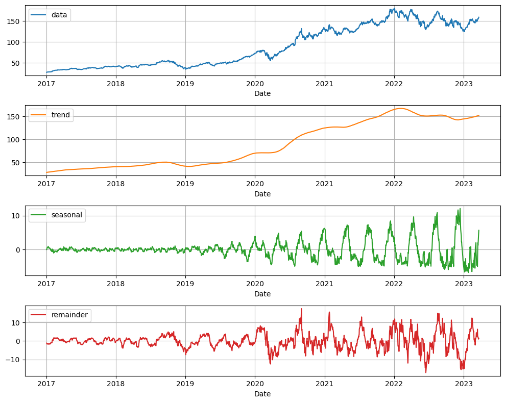
Different models manage these elements in diverse ways. Both linear models and Prophet inherently deal with all these factors. However, other models like Boosting Trees and Neural Networks necessitate clear data transformation and feature creation.

A common strategy post-decomposition is to separately model each constituent. After deriving independent predictions for each component, these can be merged to generate the ultimate forecast. This method enables a more detailed examination of time series data and frequently results in superior predictive outcomes.

Transforming Time Series Data

Frequently, transformations are utilized on time series data to stabilize variability, diminish outlier effects, enhance forecasting accuracy, and facilitate modeling. Some prevalent transformation types are:

Differencing

This transformation is a process where the preceding value (t-1) is deducted from the current value (t). Its primary function is to eliminate trend and seasonality, thus rendering the data stationary—a prerequisite for specific time series models such as ARIMA. The diff() function in pandas can be employed to perform differencing in Python:

import pandas as pd

df['diff'] = df['col'].diff()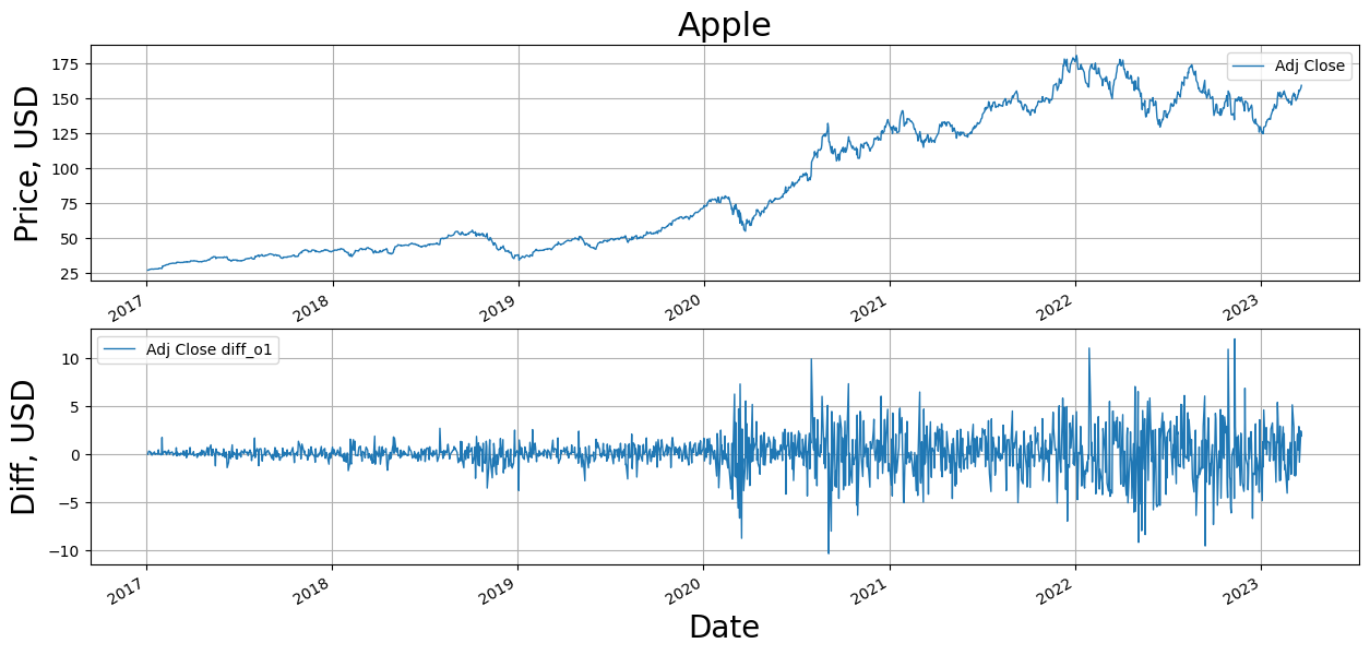

Log Transformation

Log transformation is beneficial when working with data that displays exponential growth or possesses multiplicative seasonality. This transformation aids in stabilizing variance and mitigating heteroscedasticity. The numpy library in Python can be used to execute a log transformation.

import numpy as np

df['log_col'] = np.log(df['col'])

Square Root Transformation

 The square root transformation aids in stabilizing variance and reducing the influence of extreme values or outliers. This transformation can be accomplished using numpy.

df['sqrt_col'] = np.sqrt(df['col'])

Box-Cox Transformation

This transformation encompasses both log and square root transformations as particular cases and assists in stabilizing the variance and making the data more Gaussian. The Box-Cox transformation can be denoted as the following: 

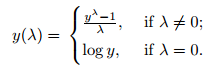
Python's SciPy library offers a function for the Box-Cox transformation.

from scipy import stats

df['boxcox_col'], lambda_param = stats.boxcox(df['col'])

It's crucial to remember post-transformation that any predictions made using the transformed data must be reverted to the original scale before interpretation. For instance, if a log transformation was employed, the predicted values should be raised to the power of e.

The selection of transformation is contingent on the specific problem, the data characteristics, and the assumptions of the ensuing modeling process. Each transformation possesses its advantages and disadvantages, and no single solution fits all scenarios. Therefore, it's advisable to experiment with different transformations and select the one that yields the best model performance.

Time Series Feature Engineering

The concept of feature engineering in the context of time series pertains to the formulation of significant predictors or features from raw temporal data to enhance the efficacy of machine learning algorithms. As opposed to problems involving tabular data, time series provides an extra dimension for maneuvering, namely, time. Here are some prominent techniques of feature engineering for time series:

• Lag Features: These encapsulate prior patterns or dependencies and are highly beneficial in solutions devised by shifting the time series data by a designated number of steps (delays).
• Rolling and Expanding Window Statistics: These techniques calculate summary metrics (like average, median, and standard deviation) over a shifting or growing window of time, helping to spot local trends and patterns.
• Seasonal and Trend Features: These assist in portraying the behavior of individual components within the model.
• Date/Time-Based Features: Specifics such as the time of day, day of the week, month, or fiscal quarter can aid in identifying repeated patterns within the data.
• Fourier Transforms: These transformations can help in discovering recurrent patterns in the data.

Employing Derivatives in Time Series Analysis

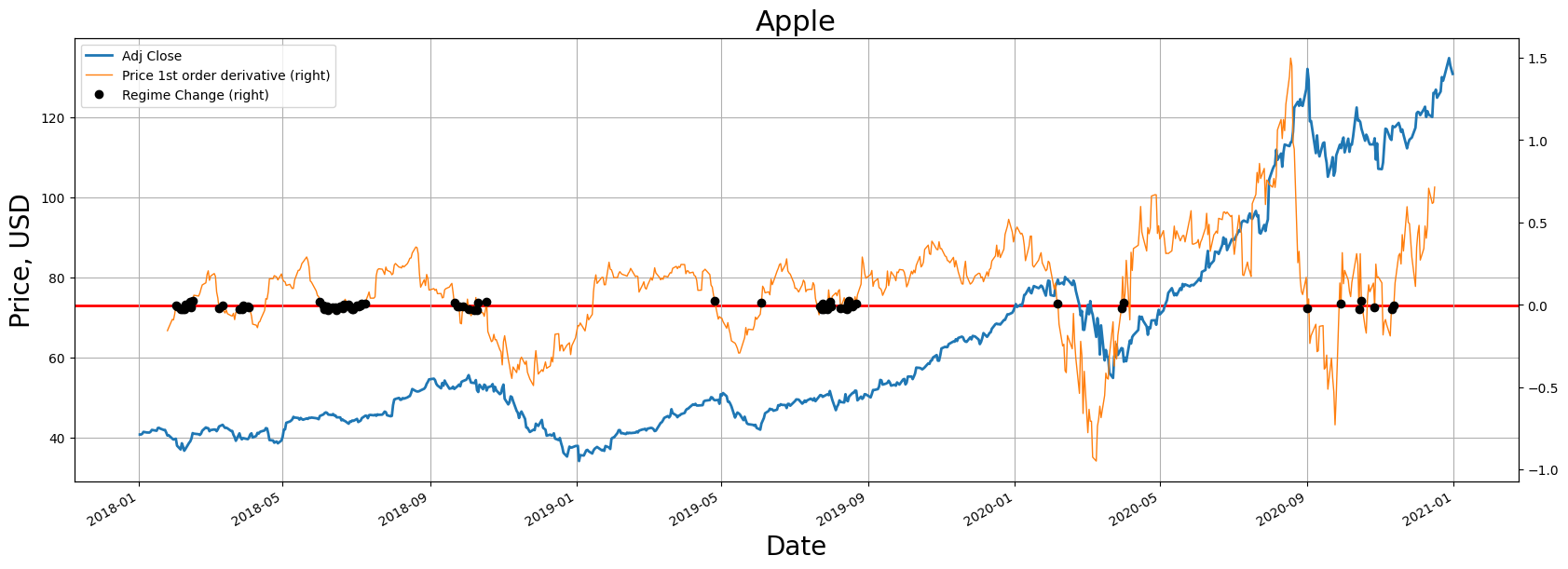
In time series analysis, derivatives denote the speed at which a time series variable alters over time. They record the changes in a variable's value over a period and can be utilized as attributes in time series evaluation or machine learning models, as they convey insights about underlying trends, cyclical changes, and additional patterns in the data. Here's a look at how derivatives can serve as attributes in time series evaluation:

• Primary Derivative: This illustrates the immediate rate of change of a variable concerning time. It aids in discerning the direction and size of the trend in the data.
• Secondary Derivative: This signifies the speed of change of the primary derivative. It assists in identifying speed-up or slow-down in the trend and pinpointing inflection points.
• Seasonal Derivatives: These derivatives are useful in identifying cyclical fluctuations in the data.
• Cross-Derivative: This is beneficial in discerning the impact of paired variables.

Time Series Modeling

Establishing a performance benchmark with baseline models is an essential process in time series forecasting, enabling the evaluation of more advanced models. Baseline models such as Exponential Smoothing, ARIMA, and Prophet remain highly effective.

Exponential Smoothing

In this instance, we'll employ the Holt-Winters method of exponential smoothing, which is designed to manage trends and seasonality. Thestatsmodels library is where this method can be found.

from statsmodels.tsa.api import ExponentialSmoothing

# Assume 'df' is a pandas DataFrame and 'col' is the time series to be forecasted
y = df['col']

# Fit the model
model = ExponentialSmoothing(y, seasonal_periods=12, trend='add', seasonal='add')
model_fit = model.fit()

# Forecast the next 5 periods
forecast = model_fit.forecast(5)

ARIMA

The AutoRegressive Integrated Moving Average (ARIMA) is a widely-used technique for predicting univariate time series data. You can find an implementation of ARIMA in the statsmodels library.

from statsmodels.tsa.arima.model import ARIMA

# Fit the model
model = ARIMA(y, order=(1,1,1))  # (p, d, q) parameters
model_fit = model.fit()

# Forecast the next 5 periods
forecast = model_fit.forecast(steps=5)

The parameters (p, d, q) correspond to the autoregressive, integrated, and moving average portions of the model, respectively.

Prophet

Prophet is a forecasting approach for time series data built around an additive model that accommodates non-linear trends with daily, weekly, and yearly seasonality and holiday effects. Facebook is behind its development.

from fbprophet import Prophet

# The input to Prophet is always a DataFrame with two columns: ds and y.
df = df.rename(columns={'date': 'ds', 'col': 'y'})

# Fit the model
model = Prophet()
model.fit(df)

# Create DataFrame for future predictions
future = model.make_future_dataframe(periods=5)

# Forecast the next 5 periods
forecast = model.predict(future)

In these examples, model parameters like the ARIMA model's order or the type of trend and seasonality in the Exponential Smoothing model are chosen somewhat arbitrarily. In a real-world scenario, you'd apply model diagnostics, cross-validation, and potentially grid search to determine the optimal parameters for your specific dataset.

Moreover, new libraries such as Nixlab offer a variety of built-in models that provide alternative viewpoints. Nevertheless, as baseline models, these methods serve as an excellent starting point for time series forecasting and accommodate a broad spectrum of time series characteristics.

Once you have some baseline scores, you can then explore advanced models such as boosting trees, Neural Networks (NNs), N-BEATS, and Temporal Fusion Transformers (TFT).

Gradient Boosting

In the domain of time series analysis, gradient boosting stands out due to its ability to make no presumptions about the data distribution or the interconnections among variables. This attribute renders it highly adaptable and proficient at handling intricate, non-linear associations typically found in time series data.

Though employing gradient boosting for time series prediction isn't as intuitive as conventional models like ARIMA, its efficacy remains high. The trick lies in structuring the prediction issue as a supervised learning problem, generating lagged features that encapsulate the temporal interdependencies in the data.

Here's an illustration of utilizing the XGBoost library, a highly optimized variant of gradient boosting, for time series prediction:

import xgboost as xgb
from sklearn.metrics import mean_squared_error

# Assume 'X_train', 'y_train', 'X_test', and 'y_test' are your training and test datasets

# Convert datasets into DMatrix (optimized data structure for XGBoost)
dtrain = xgb.DMatrix(X_train, label=y_train)
dtest = xgb.DMatrix(X_test)

# Define the model parameters
params = {
    'max_depth': 3,
    'eta': 0.01,
    'objective': 'reg:squarederror',
    'eval_metric': 'rmse'
}

# Train the model
model = xgb.train(params, dtrain, num_boost_round=1000)

# Make predictions
y_pred = model.predict(dtest)

# Evaluate the model
mse = mean_squared_error(y_test, y_pred)
print(f'Test RMSE: {np.sqrt(mse)}')

Recurrent Neural Networks (RNNs)

For RNNs, we will employ the LSTM (Long Short-Term Memory) version, renowned for capturing long-lasting dependencies and having lower susceptibility to the vanishing gradient issue.

import torch
from torch import nn

# Assume 'X_train' and 'y_train' are your training dataset
# 'n_features' is the number of input features
# 'n_steps' is the number of time steps in each sample

X_train = torch.tensor(X_train, dtype=torch.float32)
y_train = torch.tensor(y_train, dtype=torch.float32)

class RNN(nn.Module):
    def __init__(self, input_size, hidden_size, output_size):
        super(RNN, self).__init__()
        self.hidden_size = hidden_size
        self.rnn = nn.RNN(input_size, hidden_size, batch_first=True)
        self.fc = nn.Linear(hidden_size, output_size)
        
    def forward(self, x):
        x, _ = self.rnn(x)
        x = self.fc(x[:, -1, :])  # we only want the last time step
        return x

# Define the model
model = RNN(n_features, 50, 1)

# Define loss and optimizer
criterion = nn.MSELoss()
optimizer = torch.optim.Adam(model.parameters(), lr=0.01)

# Training loop
for epoch in range(200):
    model.train()
    output = model(X_train)
    loss = criterion(output, y_train)
    
    optimizer.zero_grad()
    loss.backward()
    optimizer.step()

# Make a prediction
model.eval()
x_input = ...  # some new input data
x_input = torch.tensor(x_input, dtype=torch.float32)
x_input = x_input.view((1, n_steps, n_features))
yhat = model(x_input)

N-BEATS

N-BEATS, a cutting-edge model for univariate time series prediction, is incorporated in the PyTorch-based pytorch-forecasting package.

from pytorch_forecasting import TimeSeriesDataSet, NBeats

# Assume 'data' is a pandas DataFrame containing your time series data
# 'group_ids' is the column(s) that identifies each time series
# 'target' is the column you want to forecast

# Create the dataset
max_encoder_length = 36
max_prediction_length = 6
training_cutoff = data["time_idx"].max() - max_prediction_length
context_length = max_encoder_length
prediction_length = max_prediction_length

training = TimeSeriesDataSet(
    data[lambda x: x.time_idx <= training_cutoff],
    time_idx="time_idx",
    target="target",
    group_ids=["group_ids"],
    max_encoder_length=context_length,
    max_prediction_length=prediction_length,
)

# Create the dataloaders
train_dataloader = training.to_dataloader(train=True, batch_size=128, num_workers=0)

# Define the model
pl.seed_everything(42)
trainer = pl.Trainer(gpus=0, gradient_clip_val=0.1)
net = NBeats.from_dataset(training, learning_rate=3e-2, weight_decay=1e-2, widths=[32, 512], backcast_loss_ratio=1.0)

# Fit the model
trainer.fit(
    net,
    train_dataloader=train_dataloader,
)

# Predict
raw_predictions, x = net.predict(val_dataloader, return_x=True)

Temporal Fusion Transformers (TFT)

TFT, another robust model adept at handling multivariate time series and meta-data, is also included in the pytorch-forecasting package.

Boosting trees primarily undertake most tasks due to their scalability and robust performance. Nevertheless, given sufficient time and resources, Recurrent Neural Networks (RNNs), N-BEATS, and TFT have demonstrated impressive performance in time series tasks, in spite of their significant computational demands and particular scalability.

# Import libraries
import torch
import pandas as pd
from pytorch_forecasting import TimeSeriesDataSet, TemporalFusionTransformer, Baseline, Trainer
from pytorch_forecasting.metrics import SMAPE
from pytorch_forecasting.data.examples import get_stallion_data

# Load example data
data = get_stallion_data()
data["time_idx"] = data["date"].dt.year * 12 + data["date"].dt.month
data["time_idx"] -= data["time_idx"].min()

# Define dataset
max_prediction_length = 6
max_encoder_length = 24
training_cutoff = data["time_idx"].max() - max_prediction_length

context_length = max_encoder_length
prediction_length = max_prediction_length

training = TimeSeriesDataSet(
    data[lambda x: x.time_idx <= training_cutoff],
    time_idx="time_idx",
    target="volume",
    group_ids=["agency"],
    min_encoder_length=context_length,
    max_encoder_length=context_length,
    min_prediction_length=prediction_length,
    max_prediction_length=prediction_length,
    static_categoricals=["agency"],
    static_reals=["avg_population_2017"],
    time_varying_known_categoricals=["month"],
    time_varying_known_reals=["time_idx", "minimum", "mean", "maximum"],
    time_varying_unknown_categoricals=[],
    time_varying_unknown_reals=["volume"],
)

validation = TimeSeriesDataSet.from_dataset(training, data, min_prediction_idx=training_cutoff + 1)

# Create dataloaders
batch_size = 16
train_dataloader = training.to_dataloader(train=True, batch_size=batch_size, num_workers=0)
val_dataloader = validation.to_dataloader(train=False, batch_size=batch_size * 10, num_workers=0)

# Define model and trainer
pl.seed_everything(42)
trainer = Trainer(
    gpus=0,
    # clipping gradients is a hyperparameter and important to prevent divergance
    # of the gradient for recurrent neural networks
    gradient_clip_val=0.1,
)

tft = TemporalFusionTransformer.from_dataset(
    training,
    learning_rate=0.03,
    hidden_size=16,
    lstm_layers=1,
    dropout=0.1,
    hidden_continuous_size=8,
    output_size=7,  # 7 quantiles by default
    loss=SMAPE(),
    log_interval=10,
    reduce_on_plateau_patience=4,
)

# Fit the model
trainer.fit(
    tft,
    train_dataloader=train_dataloader,
    val_dataloaders=val_dataloader,
)

# Evaluate the model
raw_predictions, x = tft.predict(val_dataloader, mode="raw", return_x=True)

Conclusion

In summary, multiple strategies can enrich time series analysis. It begins with the transformation of data and tasks to glean more insights about the nature of the data, followed by integrating time into your features and outcomes. Modeling can then commence with standard baselines, proceed with, and possibly culminate with boosting without hastily implementing neural networks and transformers.

Finally, the joint application of Dickey-Fuller and Kwiatkowski-Phillips-Schmidt-Shin tests can bolster the reliability of the outcomes.

import numpy as np
import pandas as pd
from statsmodels.tsa.stattools import adfuller, kpss

# Assume 'data' is your time series data

# Dickey-Fuller test
result = adfuller(data)
print('ADF Statistic: %f' % result[0])
print('p-value: %f' % result[1])
print('Critical Values:')
for key, value in result[4].items():
    print('\t%s: %.3f' % (key, value))

# KPSS test
result = kpss(data, regression='c')
print('\nKPSS Statistic: %f' % result[0])
print('p-value: %f' % result[1])
print('Critical Values:')
for key, value in result[3].items():
    print('\t%s: %.3f' % (key, value))