Air Compressor Predictive Maintenance using Machine Learning

This study aims to use a predictive maintenance method for identifying faulty parts in an air compressor system using artificial intelligence (AI).

Traditional methods for diagnosing and maintaining air compressor systems can be time-consuming and labor-intensive. To address this issue, we can employ AI to predict potential failures and enhance the maintenance process for air compressors, ensuring optimal operation and reducing downtime.

Contents:

This example is solved with Neural Designer. To follow it step by step, you can use the free trial.

1. Application type

We will predict the bearings status in the air compressor system, so the variable to be predicted is binary (0 or 1). Therefore, this is a classification project.

The goal here is to model the bearings status based on the features of the air compressor system for its subsequent use in predictive maintenance.

2. Data set

The first step is to prepare the data set, which is the source of information for the problem. We need to configure three things here:

• Data source.
• Variables.
• Instances.

The data file predictive_maintenance_dataset.csv contains the data for the air compressor example. This dataset includes measurements made on a compressor system feeding the air line of a factory, with 17 features collected. The number of variables (columns) is 17, and the number of instances (rows) is 1000.

The features or variables are the following:

• RPM: Indicates the number of rotations per minute for the motor.
• Motor Power: Measures the power consumption of the electric motor in kilowatts.
• Torque: Provides the torque produced by the motor in Newton-meter.
• Outlet Pressure Bar: Denotes the outlet pressure of compressed air in bars.
• Air Flow: Displays the flow rate of compressed air in cubic meters per minute.
• Noise dB: Represents the noise level of the compressor system in decibels.
• Outlet Temp Shows the outlet temperature of the compressed air in degrees Celsius.
• Water Pump Outlet Pressure: Gives the outlet pressure of the water pump in bars.
• Water Inlet Temp: Specifies the inlet temperature of cooling water in degrees Celsius.
• Water Outlet Temp: Provides the outlet temperature of cooling water in degrees Celsius.
• Water Pump Power: Measures the power consumption of the water pump in kilowatts.
• Water Flow: Indicates the cooling water flow rate in cubic meters per minute.
• Oil Pump Power: This represents the power consumption of the oil pump in kilowatts.
• Oil Tank Temp: Shows the temperature of the oil tank in degrees Celsius.
• G-Acc: Gives the acceleration of the system in the X, Y, and Z directions in gravity units (g).
• H-Acc: Provides the angular acceleration of the system in the X, Y, and Z directions in radians per second squared.
• Bearings Status: Refers to the condition of the bearings in the context of air compressors. The values can be 'Ok' for properly functioning bearings or 'Noise' for bearings that may need maintenance or replacement.

All variables in the study are inputs, except for 'Bearings Status', which is the output that we aim to extract for this machine learning study. Note that 'Bearings Status' is binary.

The instances are divided into training, selection, and testing subsets. They represent a certain percentage of the original instances and are randomly split. The exact percentages depend on the chosen data split approach.

Once the data set has been set, we can perform a few related analytics. First, we check the provided information and ensure the data is quality.

The data distributions show the bearing condition percentages.

Please note that the actual distributions may vary depending on the nature of the data collected in the air compressor dataset.

The inputs-targets correlations might indicate to us which factors have a stronger influence on the exhaust valve status.

From the chart, we can identify which features have a significant influence on bearing condition. This information can help us better understand the relationships between the variables and the target in the predictive maintenance study.

3. Neural network

The second step is to choose a neural network to represent the classification function. For classification problems it is composed of:

The scaling layer contains the statistics on the input calculated form the data file and the method for scaling the input variables. Here the minimum and maximum scaling methods are set, but the mean and standard deviation scaling method produce similar results.

We set one perceptron layer, with 4 neurons as a first guess, having the hyperbolic tangent (tanh) as acitivation function.

The next figure is a diagram for the neural network used in this example.

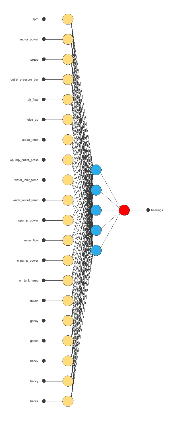
The yellow circles represent scaling neurons, the blue circles perceptron neurons, and the red circles probabilistic neurons. The number of inputs is 20, and the number of outputs is 1.

4. Training strategy

The training strategy is applied to the neural network to obtain the best possible performance. It is composed of two things:

• A loss index.
• An optimization algorithm.

The selected loss index is the normalized squared error (NSE) with L2 regularization. The normalized squared error is helpful in applications where the targets are balanced, as in this case.

The error term fits the neural network to the training instances of the data set. The regularization term makes the model more stable and improves generalization so our model will be more predictive.

The selected optimization algorithm that minimize the loss index is the quasi-Newton method.

The following chart shows how the training (blue) and selection (orange) errors decrease with the training epochs.

The final training and selection errors are training error = 0.0012 NSE (blue) and selection error = 0.0028 NSE (orange), respectively. Considering the low values of the training and selection errors, the model already demonstrates good performance.

5. Testing analysis

The next step is to perform a test analysis to validate the predictive capability of the neural network.

The next step is to perform a testing analysis to validate the predictive capability of the neural network. The testing compares the values provided by this technique to the observed values.

A good measure for the precision of a binary classification model is the ROC curve.

Our focus is on evaluating the area under the curve (AUC). A perfect classifier would have an AUC=1, which implies perfect prediction capabilities, and a random one would have AUC=0.5, indicating no better than random chance.

In this case, our model has an AUC = 0.998, which means that it has achieved practically perfect classification and prediction capabilities.

We can also look at the confusion matrix. Next, we show the elements of this matrix for a decision threshold = 0.43.

From the above confusion matrix, we can calculate the following binary classification tests:

• Classification accuracy: 99% (ratio of correctly classified samples).
• Error rate: 1% (ratio of misclassified samples).
• Sensitivity: 98.8% (percentage of actual positive classified as positive).
• Specificity: 100% (percentage of actual negative classified as negative).

6. Model deployment

Once we have tested the air compressor bearings status classification model, we can use it to evaluate the probability of a specific bearing status:

For instance, consider an air compressor with the following features:

The probability of 'Ok' for this bearings is: 100%.

We can export the mathematical expression of bearings status to facilitate the work of classification. This expression is listed below.

        scaled_rpm = (rpm-1499.52002)/707.6820068
        scaled_motor_power = (motor_power-6984.879883)/4269.279785
        scaled_torque = (torque-49.18610001)/18.70669937
        scaled_outlet_pressure_bar = (outlet_pressure_bar-4.054049969)/1.862759948
        scaled_air_flow = (air_flow-754.6740112)/442.7430115
        scaled_noise_db = (noise_db-53.41210175)/8.05535984
        scaled_outlet_temp = (outlet_temp-118.8550034)/19.1201992
        scaled_wpump_outlet_press = (wpump_outlet_press-2.7996099)/0.4552739859
        scaled_water_inlet_temp = (water_inlet_temp-83.021698)/18.64500046
        scaled_water_outlet_temp = (water_outlet_temp-96.63659668)/20.55730057
        scaled_wpump_power = (wpump_power-222.1849976)/3.774529934
        scaled_water_flow = (water_flow-53.70819855)/6.587259769
        scaled_oilpump_power = (oilpump_power-300.4840088)/0.4087029994
        scaled_oil_tank_temp = (oil_tank_temp-46.23770142)/0.1961389929
        scaled_gaccx = (gaccx-0.6017889977)/0.05871869996
        scaled_gaccy = (gaccy-0.3496670127)/0.04066679999
        scaled_gaccz = (gaccz-3.923069954)/1.610129952
        scaled_haccx = (haccx-1.101250052)/0.05854640156
        scaled_haccy = (haccy-1.350039959)/0.0408712998
        scaled_haccz = (haccz-3.49503994)/0.8176670074
        
        perceptron_layer_1_output_0 = np.tanh( 0.901466 + (scaled_rpm*0.469466) + (scaled_motor_power*0.0743812) + (scaled_torque*-0.14942) + (scaled_outlet_pressure_bar*-0.101016) + (scaled_air_flow*-0.466583) + (scaled_noise_db*-1.74041) + (scaled_outlet_temp*0.738268) + (scaled_wpump_outlet_press*0.422983) + (scaled_water_inlet_temp*0.787527) + (scaled_water_outlet_temp*0.284194) + (scaled_wpump_power*0.287301) + (scaled_water_flow*-1.30252) + (scaled_oilpump_power*0.128188) + (scaled_oil_tank_temp*0.656645) + (scaled_gaccx*-0.40253) + (scaled_gaccy*-0.0149995) + (scaled_gaccz*-0.33298) + (scaled_haccx*-0.420607) + (scaled_haccy*-0.270557) + (scaled_haccz*-0.362505) )
        perceptron_layer_1_output_1 = np.tanh( 0.32231 + (scaled_rpm*-0.0899539) + (scaled_motor_power*-0.104127) + (scaled_torque*-0.175207) + (scaled_outlet_pressure_bar*-0.122444) + (scaled_air_flow*-0.926577) + (scaled_noise_db*-1.52257) + (scaled_outlet_temp*0.865686) + (scaled_wpump_outlet_press*0.368702) + (scaled_water_inlet_temp*0.691098) + (scaled_water_outlet_temp*0.943445) + (scaled_wpump_power*0.566609) + (scaled_water_flow*-1.95932) + (scaled_oilpump_power*-0.265151) + (scaled_oil_tank_temp*0.928677) + (scaled_gaccx*-0.142292) + (scaled_gaccy*-0.126341) + (scaled_gaccz*-0.20502) + (scaled_haccx*-0.0503535) + (scaled_haccy*0.0329963) + (scaled_haccz*-0.346429) )
        perceptron_layer_1_output_2 = np.tanh( 0.886566 + (scaled_rpm*1.12165) + (scaled_motor_power*0.071234) + (scaled_torque*-0.500776) + (scaled_outlet_pressure_bar*-0.248816) + (scaled_air_flow*0.10544) + (scaled_noise_db*-2.44581) + (scaled_outlet_temp*0.681027) + (scaled_wpump_outlet_press*0.206632) + (scaled_water_inlet_temp*0.36686) + (scaled_water_outlet_temp*-0.122395) + (scaled_wpump_power*-0.119946) + (scaled_water_flow*-0.469015) + (scaled_oilpump_power*-0.0137544) + (scaled_oil_tank_temp*0.222672) + (scaled_gaccx*-0.21359) + (scaled_gaccy*0.00372433) + (scaled_gaccz*0.0634309) + (scaled_haccx*0.0104647) + (scaled_haccy*-0.090681) + (scaled_haccz*0.0527847) )
        perceptron_layer_1_output_3 = np.tanh( 1.73749 + (scaled_rpm*1.13836) + (scaled_motor_power*0.264973) + (scaled_torque*-0.45276) + (scaled_outlet_pressure_bar*-0.374484) + (scaled_air_flow*-0.911772) + (scaled_noise_db*-3.29918) + (scaled_outlet_temp*0.698172) + (scaled_wpump_outlet_press*-0.0900097) + (scaled_water_inlet_temp*0.436472) + (scaled_water_outlet_temp*0.674326) + (scaled_wpump_power*0.362162) + (scaled_water_flow*-0.995449) + (scaled_oilpump_power*0.17563) + (scaled_oil_tank_temp*0.654069) + (scaled_gaccx*-0.155581) + (scaled_gaccy*0.0901928) + (scaled_gaccz*-0.106409) + (scaled_haccx*-0.0617506) + (scaled_haccy*0.0879432) + (scaled_haccz*0.0481439) )
        perceptron_layer_1_output_4 = np.tanh( 0.0951512 + (scaled_rpm*0.143308) + (scaled_motor_power*0.251458) + (scaled_torque*0.125892) + (scaled_outlet_pressure_bar*0.151768) + (scaled_air_flow*1.4004) + (scaled_noise_db*2.28701) + (scaled_outlet_temp*-1.01135) + (scaled_wpump_outlet_press*-0.850055) + (scaled_water_inlet_temp*-1.04786) + (scaled_water_outlet_temp*-0.984143) + (scaled_wpump_power*-0.722475) + (scaled_water_flow*2.31838) + (scaled_oilpump_power*0.490667) + (scaled_oil_tank_temp*-0.791984) + (scaled_gaccx*-0.0749758) + (scaled_gaccy*-0.179896) + (scaled_gaccz*0.165896) + (scaled_haccx*-0.136697) + (scaled_haccy*-0.110109) + (scaled_haccz*0.11758) )
        
        probabilistic_layer_combinations_0 = 2.87135 +1.37052*perceptron_layer_1_output_0 -0.11211*perceptron_layer_1_output_1 +4.40601*perceptron_layer_1_output_2 +5.99676*perceptron_layer_1_output_3 +1.76189*perceptron_layer_1_output_4 
            
        bearings = 1.0/(1.0 + np.exp(-probabilistic_layer_combinations_0) )

        

References:

• Kaggle.

Related posts:

• Machine Learning Techniques for Predicting Milk Quality.