

Deep Generative Art – Monet Style Transfer with GANs (CycleGAN)
source link: https://sandipanweb.wordpress.com/2023/03/31/monet-style-transfer-with-gans-cyclegan/
Go to the source link to view the article. You can view the picture content, updated content and better typesetting reading experience. If the link is broken, please click the button below to view the snapshot at that time.

Deep Generative Art – Monet Style Transfer with GANs (CycleGAN)
This problem appeared as a project in the coursera course Deep Learning (by the University of Colorado Boulder) and also appeared in a Kaggle Competition.
Brief description of the problem and data
In this project, the goal is to build a GAN that generates 7,000 to 10,000 Monet-style images.
Computer vision has advanced tremendously in recent years and GANs are now capable of mimicking objects in a very convincing way. But creating museum-worthy masterpieces is thought of to be, well, more art than science. So can (data) science, in the form of GANs, trick classifiers into believing that we have created a true Monet? That’s the challenge we shall take on!
A GAN consists of at least two neural networks: a generator model and a discriminator model. The generator is a neural network that creates the images. For our competition, you should generate images in the style of Monet. This generator is trained using a discriminator.
The two models will work against each other, with the generator trying to trick the discriminator, and the discriminator trying to accurately classify the real vs. generated images.
Exploratory Data Analysis (EDA)
In this project we are going to use CycleGAN for style transfer. First we need to import all python packages / functions that are required (install the ones that are not already installed with pip) for building the GAN model. We shall use tensorflow / keras to train the generative model.
import numpy as npimport re, os, shutilfrom glob import globimport tqdmimport matplotlib.pylab as plt# for building the modelimport tensorflow as tfimport tensorflow.keras.backend as K#! pip install tensorflow_addonsimport tensorflow_addons as tfaimport tensorflow_datasets as tfdsfrom tensorflow import kerasfrom tensorflow.keras import layers, losses |
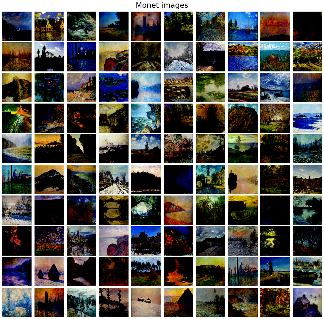
Let’s read the tfrecords and create a tensorflow ZipDataset by combining the photo and monte style images. We can see that the number of monet style images (300) is much smaller than number of photo images (7038), so the images are not paired.
def load_dataset(filenames, labeled=True, ordered=False, autotune=tf.data.experimental.AUTOTUNE):dataset = tf.data.TFRecordDataset(filenames)dataset = dataset.map(read_tfrecord, num_parallel_calls=autotune)return datasetdef decode_image(image, img_size=[256,256,3]):image = tf.image.decode_jpeg(image, channels=3)image = (tf.cast(image, tf.float32) / 127.5) - 1 image = tf.reshape(image, img_size) return imagedef read_tfrecord(example):tfrecord_format = {"image_name": tf.io.FixedLenFeature([], tf.string),"image": tf.io.FixedLenFeature([], tf.string),"target": tf.io.FixedLenFeature([], tf.string)}example = tf.io.parse_single_example(example, tfrecord_format) image = decode_image(example['image']) return imagedef count_data_items(filenames):n = [int(re.compile(r"-([0-9]*)\.").search(filename).group(1)) for filename in filenames]return np.sum(n)data_path = 'gan-getting-started'monet_filenames = tf.io.gfile.glob(str(os.path.join(data_path, 'monet_tfrec', '*.tfrec')))photo_filenames = tf.io.gfile.glob(str(os.path.join(data_path, 'photo_tfrec', '*.tfrec')))monet_ds = load_dataset(monet_filenames)photo_ds = load_dataset(photo_filenames)n_monet_samples = count_data_items(monet_filenames)n_photo_samples = count_data_items(photo_filenames)dataset = tf.data.Dataset.zip((monet_ds, photo_ds))n_monet_samples, n_photo_samples# (300, 7038) |
Let’s plot a few sample images from monet style and photo images.
def plot_images(images, title):plt.figure(figsize=(15,15))plt.subplots_adjust(0,0,1,0.95,0.05,0.05)j = 1for i in np.random.choice(len(images), 100, replace=False):plt.subplot(10,10,j), plt.imshow(images[i] / images[i].max()), plt.axis('off')j += 1plt.suptitle(title, size=25)plt.show()monet_numpy = list(monet_ds.as_numpy_iterator())plot_images(monet_numpy, 'Monet images') |
Monet Style input images
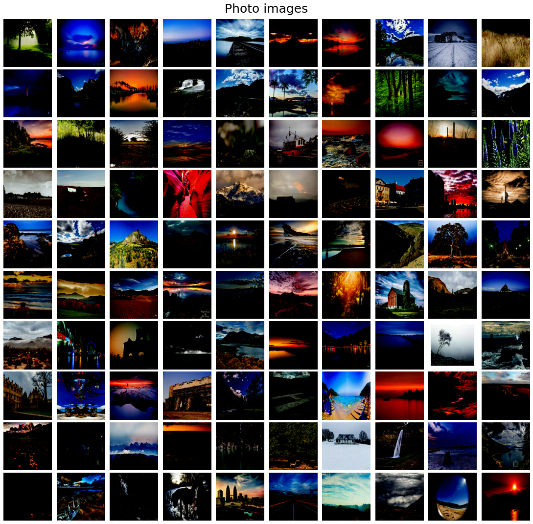
plot_images(list(photo_ds.as_numpy_iterator()), 'Photo images') |
Photo input images
Preprocessing
As can be seen, the images are transformed to have values in between [-1,1], implemented with the function decode_image() above.
Model Architecture
Paired data is harder to find in most domains, and not even possible in some, the unsupervised training capabilities of CycleGAN are quite useful, it does not require paired training data (which we don’t have in this case, we have 300 monet images and ~7k photo images). Hence, the problem can be forumulated as unpaired image-to-image translation and CycleGAN is an ideal model to be used here. We shall train the CycleGAN model on the image dataset provided (to translate from photo to monet style images) and then use the Genrator to generate monet images later. The next figure shows the architecture and the next code snippet provides the implementation:

class CycleGAN(keras.Model):def __init__(self,monet_generator,photo_generator,monet_discriminator,photo_discriminator,lambda_cycle=10,):super(CycleGAN, self).__init__()self.m_gen = monet_generatorself.p_gen = photo_generatorself.m_disc = monet_discriminatorself.p_disc = photo_discriminatorself.lambda_cycle = lambda_cycledef compile(self,m_gen_optimizer,p_gen_optimizer,m_disc_optimizer,p_disc_optimizer,gen_loss_fn,disc_loss_fn,cycle_loss_fn,identity_loss_fn):super(CycleGAN, self).compile()self.m_gen_optimizer = m_gen_optimizerself.p_gen_optimizer = p_gen_optimizerself.m_disc_optimizer = m_disc_optimizerself.p_disc_optimizer = p_disc_optimizerself.gen_loss_fn = gen_loss_fnself.disc_loss_fn = disc_loss_fnself.cycle_loss_fn = cycle_loss_fnself.identity_loss_fn = identity_loss_fndef generate(self, image):return self.m_gen(tf.expand_dims(image, axis=0), training=False)def load(self, filepath):self.m_gen.load_weights(filepath.replace('model_name', 'm_gen'), by_name=True)self.p_gen.load_weights(filepath.replace('model_name', 'p_gen'), by_name=True)self.m_disc.load_weights(filepath.replace('model_name', 'm_disc'), by_name=True)self.p_disc.load_weights(filepath.replace('model_name', 'p_disc'), by_name=True)def save(self, filepath):self.m_gen.save(filepath.replace('model_name', 'm_gen'))self.p_gen.save(filepath.replace('model_name', 'p_gen'))self.m_disc.save(filepath.replace('model_name', 'm_disc'))self.p_disc.save(filepath.replace('model_name', 'p_disc'))def train_step(self, batch_data):real_monet, real_photo = batch_datawith tf.GradientTape(persistent=True) as tape:# photo to monet back to photoreal_photo = tf.expand_dims(real_photo, axis=0)real_monet = tf.expand_dims(real_monet, axis=0)fake_monet = self.m_gen(real_photo, training=True)cycled_photo = self.p_gen(fake_monet, training=True)# monet to photo back to monetfake_photo = self.p_gen(real_monet, training=True)cycled_monet = self.m_gen(fake_photo, training=True)# generating itselfsame_monet = self.m_gen(real_monet, training=True)same_photo = self.p_gen(real_photo, training=True)# discriminator used to check, inputing real imagesdisc_real_monet = self.m_disc(real_monet, training=True)disc_real_photo = self.p_disc(real_photo, training=True)# discriminator used to check, inputing fake imagesdisc_fake_monet = self.m_disc(fake_monet, training=True)disc_fake_photo = self.p_disc(fake_photo, training=True)# evaluates generator lossmonet_gen_loss = self.gen_loss_fn(disc_fake_monet)photo_gen_loss = self.gen_loss_fn(disc_fake_photo)# evaluates total cycle consistency losstotal_cycle_loss = self.cycle_loss_fn(real_monet, cycled_monet, self.lambda_cycle) + self.cycle_loss_fn(real_photo, cycled_photo, self.lambda_cycle)# evaluates total generator losstotal_monet_gen_loss = monet_gen_loss + total_cycle_loss + self.identity_loss_fn(real_monet, same_monet, self.lambda_cycle)total_photo_gen_loss = photo_gen_loss + total_cycle_loss + self.identity_loss_fn(real_photo, same_photo, self.lambda_cycle)# evaluates discriminator lossmonet_disc_loss = self.disc_loss_fn(disc_real_monet, disc_fake_monet)photo_disc_loss = self.disc_loss_fn(disc_real_photo, disc_fake_photo)# Calculate the gradients for generator and discriminatormonet_generator_gradients = tape.gradient(total_monet_gen_loss, self.m_gen.trainable_variables)photo_generator_gradients = tape.gradient(total_photo_gen_loss, self.p_gen.trainable_variables)monet_discriminator_gradients = tape.gradient(monet_disc_loss, self.m_disc.trainable_variables)photo_discriminator_gradients = tape.gradient(photo_disc_loss, self.p_disc.trainable_variables)# Apply the gradients to the optimizerself.m_gen_optimizer.apply_gradients(zip(monet_generator_gradients, self.m_gen.trainable_variables))self.p_gen_optimizer.apply_gradients(zip(photo_generator_gradients, self.p_gen.trainable_variables))self.m_disc_optimizer.apply_gradients(zip(monet_discriminator_gradients, self.m_disc.trainable_variables))self.p_disc_optimizer.apply_gradients(zip(photo_discriminator_gradients, self.p_disc.trainable_variables))total_loss = total_monet_gen_loss + total_photo_gen_loss + monet_disc_loss + photo_disc_lossreturn {"total_loss": total_loss,"monet_gen_loss": total_monet_gen_loss,"photo_gen_loss": total_photo_gen_loss,"monet_disc_loss": monet_disc_loss,"photo_disc_loss": photo_disc_loss} |
The CycleGAN is an extension of the GAN architecture that involves the simultaneous training of two generator models and two discriminator models. The CycleGAN uses an additional extension to the architecture called cycle consistency. This is the idea that an image output by the first generator could be used as input to the second generator and the output of the second generator should match the original image.
The Discriminator is a deep convolutional neural network that performs image classification. It takes a source image as input and predicts the likelihood of whether the target image is a real or fake image. Two discriminator models are used, one for Domain-A (photos) and one for Domain-B (monets).

The generator is an encoder-decoder model architecture. The discriminator models are trained directly on real and generated images, whereas the generator models are not. The model takes a source image (e.g. a photo) and generates a target image (e.g. a monet image). It does this by first downsampling or encoding the input image down to a bottleneck layer, then interpreting the encoding with a number of ResNet layers that use skip connections, followed by a series of layers that upsample or decode the representation to the size of the output image.

def Generator(img_shape=[256, 256, 3]):inputs = layers.Input(shape=img_shape)down_stack = [downsample(64, 4, apply_instancenorm=False),downsample(128, 4),downsample(256, 4),downsample(512, 4),downsample(512, 4),downsample(512, 4),downsample(512, 4),downsample(512, 4),]up_stack = [upsample(512, 4, apply_dropout=True),upsample(512, 4, apply_dropout=True),upsample(512, 4, apply_dropout=True),upsample(512, 4),upsample(256, 4),upsample(128, 4),upsample(64, 4),]initializer = tf.random_normal_initializer(0., 0.02)last = layers.Conv2DTranspose(3, 4, strides=2, padding='same', kernel_initializer=initializer, activation='tanh')x = inputsskips = []for down in down_stack:x = down(x)skips.append(x)skips = reversed(skips[:-1])for up, skip in zip(up_stack, skips):x = up(x)x = layers.Concatenate()([x, skip])x = last(x)return keras.Model(inputs=inputs, outputs=x)def Discriminator(img_shape=[256, 256, 3]):initializer = tf.random_normal_initializer(0., 0.02)gamma_init = keras.initializers.RandomNormal(mean=0.0, stddev=0.02)inp = layers.Input(shape=img_shape, name='input_image')x = inpx = downsample(64, 4, False)(x) x = downsample(128, 4)(x) x = downsample(256, 4)(x) x = layers.ZeroPadding2D()(x) x = layers.Conv2D(512, 4, strides=1, kernel_initializer=initializer, use_bias=False)(x) x = tfa.layers.InstanceNormalization(gamma_initializer=gamma_init)(x)x = layers.LeakyReLU()(x)x = layers.ZeroPadding2D()(x) x = layers.Conv2D(1, 4, strides=1, kernel_initializer=initializer)(x) return tf.keras.Model(inputs=inp, outputs=x) |
def downsample(filters, size, apply_instancenorm=True):initializer = tf.random_normal_initializer(0., 0.02)gamma_init = keras.initializers.RandomNormal(mean=0.0, stddev=0.02)result = keras.Sequential()result.add(layers.Conv2D(filters, size, strides=2, padding='same', kernel_initializer=initializer, use_bias=False))if apply_instancenorm:result.add(tfa.layers.InstanceNormalization(gamma_initializer=gamma_init))result.add(layers.LeakyReLU())return resultdef upsample(filters, size, apply_dropout=False):initializer = tf.random_normal_initializer(0., 0.02)gamma_init = keras.initializers.RandomNormal(mean=0.0, stddev=0.02)result = keras.Sequential()result.add(layers.Conv2DTranspose(filters, size, strides=2, padding='same', kernel_initializer=initializer, use_bias=False))result.add(tfa.layers.InstanceNormalization(gamma_initializer=gamma_init))if apply_dropout:result.add(layers.Dropout(0.5))result.add(layers.ReLU())return resultdef discriminator_loss(real, generated):real_loss = losses.BinaryCrossentropy(from_logits=True, reduction=losses.Reduction.NONE)(tf.ones_like(real), real)generated_loss = losses.BinaryCrossentropy(from_logits=True, reduction=losses.Reduction.NONE)(tf.zeros_like(generated), generated)total_disc_loss = real_loss + generated_lossreturn total_disc_loss * 0.5def generator_loss(generated):return losses.BinaryCrossentropy(from_logits=True, reduction=losses.Reduction.NONE)(tf.ones_like(generated), generated)def calc_cycle_loss(real_image, cycled_image, LAMBDA):return LAMBDA * tf.reduce_mean(tf.abs(real_image - cycled_image))def identity_loss(real_image, same_image, LAMBDA):return LAMBDA * 0.5 * tf.reduce_mean(tf.abs(real_image - same_image)) |
img_shape = [256, 256, 3]model = CycleGAN(monet_generator=Generator(img_shape),photo_generator=Generator(img_shape),monet_discriminator=Discriminator(img_shape),photo_discriminator=Discriminator(img_shape),lambda_cycle=10)model.compile(m_gen_optimizer=tf.keras.optimizers.Adam(1e-4, beta_1=0.5),p_gen_optimizer=tf.keras.optimizers.Adam(1e-4, beta_1=0.5),m_disc_optimizer=tf.keras.optimizers.Adam(1e-4, beta_1=0.5),p_disc_optimizer=tf.keras.optimizers.Adam(1e-4, beta_1=0.5),gen_loss_fn=generator_loss,disc_loss_fn=discriminator_loss,cycle_loss_fn=calc_cycle_loss,identity_loss_fn=identity_loss) |
Results and Analysis
Let’s train the GAN model (both the generators and discriminators simultaneously) for 50 epochs.
# Train the modelbatch_size = 32#tf.config.run_functions_eagerly(True)#tf.get_logger().setLevel('INFO')epochs = 50history = model.fit(dataset, epochs=epochs, batch_size=batch_size)Epoch 1/502023-03-27 19:18:41.116027: E tensorflow/core/grappler/optimizers/meta_optimizer.cc:954] layout failed: INVALID_ARGUMENT: Size of values 0 does not match size of permutation 4 @ fanin shape inmodel/sequential_8/dropout/dropout_2/SelectV2-2-TransposeNHWCToNCHW-LayoutOptimizer300/300 [==============================] - 178s 442ms/step - total_loss: 13.5143 - monet_gen_loss: 6.0788 - photo_gen_loss: 6.2427 - monet_disc_loss: 0.6130 - photo_disc_loss: 0.5799Epoch 2/50300/300 [==============================] - 132s 440ms/step - total_loss: 9.6236 - monet_gen_loss: 4.1237 - photo_gen_loss: 4.3565 - monet_disc_loss: 0.6405 - photo_disc_loss: 0.5029Epoch 3/50300/300 [==============================] - 132s 440ms/step - total_loss: 9.1091 - monet_gen_loss: 3.8061 - photo_gen_loss: 4.2105 - monet_disc_loss: 0.6381 - photo_disc_loss: 0.4545Epoch 4/50300/300 [==============================] - 132s 440ms/step - total_loss: 9.0574 - monet_gen_loss: 3.8176 - photo_gen_loss: 4.1377 - monet_disc_loss: 0.5952 - photo_disc_loss: 0.5070Epoch 5/50300/300 [==============================] - 132s 440ms/step - total_loss: 9.0721 - monet_gen_loss: 3.8688 - photo_gen_loss: 4.1645 - monet_disc_loss: 0.5462 - photo_disc_loss: 0.4925Epoch 6/50300/300 [==============================] - 132s 440ms/step - total_loss: 9.1115 - monet_gen_loss: 3.8860 - photo_gen_loss: 4.1123 - monet_disc_loss: 0.5778 - photo_disc_loss: 0.5354Epoch 7/50300/300 [==============================] - 132s 439ms/step - total_loss: 8.9233 - monet_gen_loss: 3.7933 - photo_gen_loss: 3.9551 - monet_disc_loss: 0.5987 - photo_disc_loss: 0.5761Epoch 8/50300/300 [==============================] - 132s 440ms/step - total_loss: 8.7080 - monet_gen_loss: 3.6934 - photo_gen_loss: 3.8289 - monet_disc_loss: 0.6077 - photo_disc_loss: 0.5780Epoch 9/50300/300 [==============================] - 132s 440ms/step - total_loss: 8.5513 - monet_gen_loss: 3.6243 - photo_gen_loss: 3.7549 - monet_disc_loss: 0.5994 - photo_disc_loss: 0.5727Epoch 10/50300/300 [==============================] - 132s 440ms/step - total_loss: 8.4467 - monet_gen_loss: 3.5701 - photo_gen_loss: 3.7059 - monet_disc_loss: 0.6021 - photo_disc_loss: 0.5686Epoch 11/50300/300 [==============================] - 132s 440ms/step - total_loss: 8.3335 - monet_gen_loss: 3.5100 - photo_gen_loss: 3.6443 - monet_disc_loss: 0.6047 - photo_disc_loss: 0.5744Epoch 12/50300/300 [==============================] - 132s 440ms/step - total_loss: 8.1454 - monet_gen_loss: 3.3979 - photo_gen_loss: 3.5508 - monet_disc_loss: 0.6197 - photo_disc_loss: 0.5770Epoch 13/50300/300 [==============================] - 132s 440ms/step - total_loss: 7.9934 - monet_gen_loss: 3.3216 - photo_gen_loss: 3.4639 - monet_disc_loss: 0.6189 - photo_disc_loss: 0.5889Epoch 14/50300/300 [==============================] - 132s 440ms/step - total_loss: 7.8940 - monet_gen_loss: 3.2744 - photo_gen_loss: 3.4177 - monet_disc_loss: 0.6144 - photo_disc_loss: 0.5875Epoch 15/50300/300 [==============================] - 132s 440ms/step - total_loss: 7.8149 - monet_gen_loss: 3.2327 - photo_gen_loss: 3.3816 - monet_disc_loss: 0.6144 - photo_disc_loss: 0.5862Epoch 16/50300/300 [==============================] - 132s 440ms/step - total_loss: 7.7611 - monet_gen_loss: 3.2000 - photo_gen_loss: 3.3537 - monet_disc_loss: 0.6176 - photo_disc_loss: 0.5898Epoch 17/50300/300 [==============================] - 132s 440ms/step - total_loss: 7.7349 - monet_gen_loss: 3.1919 - photo_gen_loss: 3.3390 - monet_disc_loss: 0.6143 - photo_disc_loss: 0.5897Epoch 18/50300/300 [==============================] - 132s 439ms/step - total_loss: 7.6678 - monet_gen_loss: 3.1610 - photo_gen_loss: 3.2970 - monet_disc_loss: 0.6160 - photo_disc_loss: 0.5938Epoch 19/50300/300 [==============================] - 132s 440ms/step - total_loss: 7.6531 - monet_gen_loss: 3.1560 - photo_gen_loss: 3.2872 - monet_disc_loss: 0.6158 - photo_disc_loss: 0.5941Epoch 20/50300/300 [==============================] - 132s 440ms/step - total_loss: 7.5918 - monet_gen_loss: 3.1216 - photo_gen_loss: 3.2546 - monet_disc_loss: 0.6182 - photo_disc_loss: 0.5974Epoch 21/50300/300 [==============================] - 132s 439ms/step - total_loss: 7.5678 - monet_gen_loss: 3.1125 - photo_gen_loss: 3.2480 - monet_disc_loss: 0.6141 - photo_disc_loss: 0.5932Epoch 22/50300/300 [==============================] - 132s 439ms/step - total_loss: 7.5094 - monet_gen_loss: 3.0878 - photo_gen_loss: 3.2083 - monet_disc_loss: 0.6158 - photo_disc_loss: 0.5975Epoch 23/50300/300 [==============================] - 132s 439ms/step - total_loss: 7.5019 - monet_gen_loss: 3.0877 - photo_gen_loss: 3.2045 - monet_disc_loss: 0.6138 - photo_disc_loss: 0.5958Epoch 24/50300/300 [==============================] - 132s 440ms/step - total_loss: 7.4443 - monet_gen_loss: 3.0563 - photo_gen_loss: 3.1699 - monet_disc_loss: 0.6180 - photo_disc_loss: 0.6001Epoch 25/50300/300 [==============================] - 132s 439ms/step - total_loss: 7.4156 - monet_gen_loss: 3.0429 - photo_gen_loss: 3.1655 - monet_disc_loss: 0.6165 - photo_disc_loss: 0.5907Epoch 26/50300/300 [==============================] - 132s 440ms/step - total_loss: 7.3863 - monet_gen_loss: 3.0236 - photo_gen_loss: 3.1437 - monet_disc_loss: 0.6213 - photo_disc_loss: 0.5977Epoch 27/50300/300 [==============================] - 132s 440ms/step - total_loss: 7.3447 - monet_gen_loss: 3.0054 - photo_gen_loss: 3.1185 - monet_disc_loss: 0.6231 - photo_disc_loss: 0.5977Epoch 28/50300/300 [==============================] - 132s 440ms/step - total_loss: 7.3085 - monet_gen_loss: 2.9852 - photo_gen_loss: 3.0985 - monet_disc_loss: 0.6254 - photo_disc_loss: 0.5994Epoch 29/50300/300 [==============================] - 132s 440ms/step - total_loss: 7.2748 - monet_gen_loss: 2.9651 - photo_gen_loss: 3.0832 - monet_disc_loss: 0.6306 - photo_disc_loss: 0.5960Epoch 30/50300/300 [==============================] - 132s 440ms/step - total_loss: 7.2610 - monet_gen_loss: 2.9589 - photo_gen_loss: 3.0837 - monet_disc_loss: 0.6276 - photo_disc_loss: 0.5908Epoch 31/50300/300 [==============================] - 132s 440ms/step - total_loss: 7.1940 - monet_gen_loss: 2.9234 - photo_gen_loss: 3.0399 - monet_disc_loss: 0.6340 - photo_disc_loss: 0.5967Epoch 32/50300/300 [==============================] - 132s 440ms/step - total_loss: 7.1518 - monet_gen_loss: 2.9051 - photo_gen_loss: 3.0160 - monet_disc_loss: 0.6356 - photo_disc_loss: 0.5952Epoch 33/50300/300 [==============================] - 132s 439ms/step - total_loss: 7.1283 - monet_gen_loss: 2.8942 - photo_gen_loss: 3.0005 - monet_disc_loss: 0.6368 - photo_disc_loss: 0.5969Epoch 34/50300/300 [==============================] - 132s 439ms/step - total_loss: 7.0966 - monet_gen_loss: 2.8813 - photo_gen_loss: 2.9824 - monet_disc_loss: 0.6379 - photo_disc_loss: 0.5950Epoch 35/50300/300 [==============================] - 132s 439ms/step - total_loss: 7.0460 - monet_gen_loss: 2.8441 - photo_gen_loss: 2.9676 - monet_disc_loss: 0.6409 - photo_disc_loss: 0.5934Epoch 36/50300/300 [==============================] - 132s 439ms/step - total_loss: 6.9889 - monet_gen_loss: 2.8174 - photo_gen_loss: 2.9290 - monet_disc_loss: 0.6417 - photo_disc_loss: 0.6008Epoch 37/50300/300 [==============================] - 132s 439ms/step - total_loss: 6.9392 - monet_gen_loss: 2.7863 - photo_gen_loss: 2.9042 - monet_disc_loss: 0.6431 - photo_disc_loss: 0.6055Epoch 38/50300/300 [==============================] - 132s 440ms/step - total_loss: 6.9482 - monet_gen_loss: 2.8005 - photo_gen_loss: 2.9125 - monet_disc_loss: 0.6349 - photo_disc_loss: 0.6004Epoch 39/50300/300 [==============================] - 132s 440ms/step - total_loss: 6.9012 - monet_gen_loss: 2.7681 - photo_gen_loss: 2.8925 - monet_disc_loss: 0.6363 - photo_disc_loss: 0.6043Epoch 40/50300/300 [==============================] - 132s 440ms/step - total_loss: 6.7845 - monet_gen_loss: 2.7000 - photo_gen_loss: 2.8238 - monet_disc_loss: 0.6453 - photo_disc_loss: 0.6154Epoch 41/50300/300 [==============================] - 132s 440ms/step - total_loss: 6.7913 - monet_gen_loss: 2.6840 - photo_gen_loss: 2.8536 - monet_disc_loss: 0.6443 - photo_disc_loss: 0.6094Epoch 42/50300/300 [==============================] - 132s 440ms/step - total_loss: 6.6722 - monet_gen_loss: 2.6384 - photo_gen_loss: 2.7718 - monet_disc_loss: 0.6458 - photo_disc_loss: 0.6163Epoch 43/50300/300 [==============================] - 132s 440ms/step - total_loss: 6.7128 - monet_gen_loss: 2.6721 - photo_gen_loss: 2.7917 - monet_disc_loss: 0.6393 - photo_disc_loss: 0.6097Epoch 44/50300/300 [==============================] - 132s 439ms/step - total_loss: 6.6979 - monet_gen_loss: 2.6490 - photo_gen_loss: 2.8041 - monet_disc_loss: 0.6406 - photo_disc_loss: 0.6041Epoch 45/50300/300 [==============================] - 132s 439ms/step - total_loss: 6.9362 - monet_gen_loss: 2.8560 - photo_gen_loss: 2.9042 - monet_disc_loss: 0.5885 - photo_disc_loss: 0.5875Epoch 46/50300/300 [==============================] - 132s 439ms/step - total_loss: 6.8214 - monet_gen_loss: 2.7380 - photo_gen_loss: 2.8306 - monet_disc_loss: 0.6469 - photo_disc_loss: 0.6059Epoch 47/50300/300 [==============================] - 132s 440ms/step - total_loss: 6.6745 - monet_gen_loss: 2.6516 - photo_gen_loss: 2.7894 - monet_disc_loss: 0.6332 - photo_disc_loss: 0.6002Epoch 48/50300/300 [==============================] - 132s 439ms/step - total_loss: 6.7603 - monet_gen_loss: 2.7036 - photo_gen_loss: 2.8374 - monet_disc_loss: 0.6253 - photo_disc_loss: 0.5939Epoch 49/50300/300 [==============================] - 132s 440ms/step - total_loss: 6.8899 - monet_gen_loss: 2.8052 - photo_gen_loss: 2.9074 - monet_disc_loss: 0.6024 - photo_disc_loss: 0.5748Epoch 50/50300/300 [==============================] - 132s 439ms/step - total_loss: 6.7139 - monet_gen_loss: 2.6874 - photo_gen_loss: 2.8110 - monet_disc_loss: 0.6241 - photo_disc_loss: 0.5913 |
Let’s save the model.
model.save('cyclegan_100.h5') |
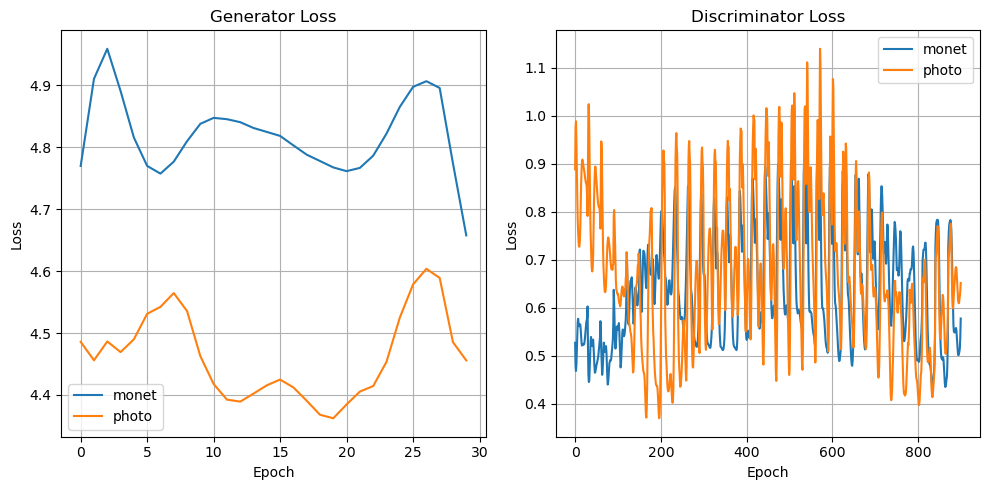
Let’s plot the loss for the generators and discriminators, for generators we plot the mean loss.
history.history.keys()# dict_keys(['total_loss', 'monet_gen_loss', 'photo_gen_loss', 'monet_disc_loss', 'photo_disc_loss']) |
def plot_hist(hist):plt.figure(figsize=(10,5))plt.subplot(121)#plt.plot(np.mean(hist.history['monet_gen_loss'][0][0], axis=1))#plt.plot(np.mean(hist.history['photo_gen_loss'][0][0], axis=1)) plt.plot(hist.history['monet_gen_loss'][0][0].flatten())plt.plot(hist.history['photo_gen_loss'][0][0].flatten()) plt.legend(["monet","photo"])plt.title('Generator Loss')plt.ylabel("Loss")plt.xlabel("Epoch")plt.grid()plt.subplot(122)plt.plot(hist.history['monet_disc_loss'][0][0].flatten())plt.plot(hist.history['photo_disc_loss'][0][0].flatten())plt.title("Discriminator Loss")plt.ylabel("Loss")plt.xlabel("Epoch")plt.grid()plt.legend(["monet","photo"])plt.tight_layout()plt.show()plot_hist(history) |
Finally, let’s use the generated to generate ~7k images and save / submit the notebook to kaggle.
! mkdir ../imagesdef generate(dataset):dataset_iter = iter(dataset)out_dir = '../images/'for i in tqdm.tqdm(range(n_photo_samples)):# Get the image from the dataset iteratorimg = next(dataset_iter)prediction = model.generate(img)prediction = tf.squeeze(prediction).numpy()prediction = (prediction * 127.5 + 127.5).astype(np.uint8) plt.imsave(os.path.join(out_dir, 'image_{:04d}.jpg'.format(i)), prediction)generate(photo_ds)shutil.make_archive("/kaggle/working/images", 'zip', "/kaggle/images") |
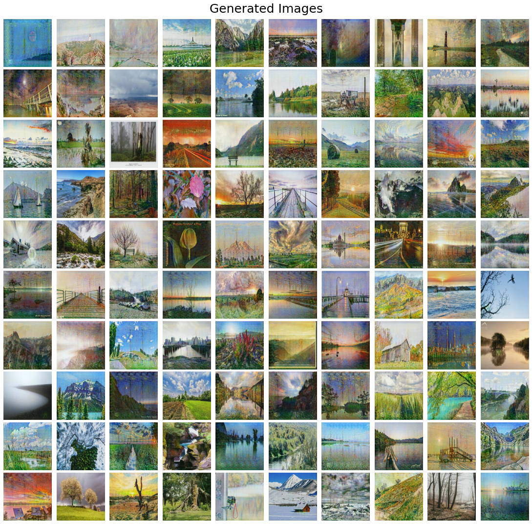
The next figure shows few of the images generated.
plot_images([plt.imread(f) for f in glob('out/*.jpg')[:200]], 'Generated Images') |

Git Repository
https://github.com/sandipan/Monet-Style-Transfer-with-GANs-Kaggle-Mini-Project
Kaggle Notebook
https://www.kaggle.com/code/sandipanumbc/monet-style-transfer-with-cyclegan
Conclusion
As we can see from the above results, the CycleGAN does a pretty good job in generating the monet-style images from photos. The model was trained for 50 epochs, it seems that losses will decrease further if increased for more epochs (e.g., 100), we can get a better model.
Kaggle uses an evaluation metric called MiFID (Memorization-informed Fréchet Inception Distance) score to evaluate the quality of generated images. The score obtained on Kaggle is ~54.18 and the leaderboard position is 49, as shown in the following screenshots.


Recommend
About Joyk
Aggregate valuable and interesting links.
Joyk means Joy of geeK