

What Is Iterative Refinement?
source link: https://nhigham.com/2023/03/13/what-is-iterative-refinement/
Go to the source link to view the article. You can view the picture content, updated content and better typesetting reading experience. If the link is broken, please click the button below to view the snapshot at that time.

What Is Iterative Refinement?
Iterative refinement is a method for improving the quality of an approximate solution 


- Compute the residual
.
- Solve
.
- Update
.
- Repeat from step 1 if necessary.
At first sight, this algorithm seems as expensive as solving for the original 


Turning to the error, with a stable LU factorization the initial 

where 


But if the solver cannot compute the initial
The simplest answer is that when iterative refinement was first used on digital computers the residual 

Here is a MATLAB example, where the working precision is single and residuals are computed in double precision.
n = 8; A = single(gallery('frank',n)); xact = ones(n,1);
b = A*xact; % b is formed exactly for small n.
x = A\b;
fprintf('Initial_error = %4.1e\n', norm(x - xact,inf))
r = single( double(b) - double(A)*double(x) );
d = A\r;
x = x + d;
fprintf('Second error  = %4.1e\n', norm(x - xact,inf))
The output is
Initial_error = 9.1e-04
Second error  = 6.0e-08
which shows that after just one step the error has been brought down from 

Fixed Precision Iterative Refinement
By the 1970s, computers had started to lose the ability to cheaply accumulate inner products in extra precision, and extra precision could not be programmed portably in software. It was discovered, though, that even if iterative refinement is run entirely in one precision it can bring benefits when
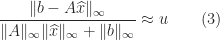
- if the solver is somewhat numerically unstable the instability is cured by the refinement, in that a relative residual satisfying
is produced, and
- a relative error satisfying
is produced, where

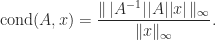
The bound (4) is stronger than (1) because 

Low Precision Factorization
In the 2000s processors became available in which 32-bit single precision arithmetic ran at twice the speed of 64-bit double precision arithmetic. A new usage of iterative refinement was developed in which the working precision is double precision and a double precision matrix
- Factorize
- Solve
by substitution in single precision, obtaining
- Compute the residual
- Solve
in single precision.
- Update
- Repeat from step 3 if necessary.
Since most of the work is in the single precision factorization, this algorithm is potentially twice as fast as solving 
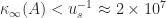
GRMES-IR
A way to weaken this restriction on

by GMRES (a Krylov subspace iterative method) in double precision. Within GMRES, 

This GMRES-based iterative refinement becomes particularly advantageous when the fast half precision arithmetic now available in hardware is used within the LU factorization, and one can use three or more precisions in the algorithm in order to balance speed, accuracy, and the range of problems that can be solved.
Finally, we note that iterative refinement can also be applied to least squares problems, eigenvalue problems, and the singular value decomposition. See Higham and Mary (2022) for details and references.
References
We give five references, which contain links to the earlier literature.
- Erin Carson and Nicholas J. Higham. Accelerating the Solution of Linear Systems by Iterative Refinement in Three Precisions. SIAM J. Sci. Comput., 40(2):A817–A847,2018.
- Azzam Haidar, Harun Bayraktar, Stanimire Tomov, Jack Dongarra, and Nicholas J. Higham. Mixed-Precision Iterative Refinement Using Tensor Cores on GPUs to Accelerate Solution Of linear systems. Proc. Roy. Soc. London A, 476(2243):20200110, 2020.
- Nicholas J. Higham and Theo Mary. Mixed Precision Algorithms in Numerical Linear Algebra. Acta Numerica, 31:347–414, 2022.
- Nicholas J. Higham and Dennis Sherwood, How to Boost Your Creativity, SIAM News, 55(5):1, 3, 2022. (Explains how developments in iterative refinement 1948–2022 correspond to asking “how might this be different” about each aspect of the algorithm.)
- Julie Langou, Julien Langou, Piotr Luszczek, Jakub Kurzak, Alfredo Buttari, and Jack Dongarra. Exploiting the Performance of 32 Bit Floating Point Arithmetic in Obtaining 64 Bit Accuracy (Revisiting Iterative Refinement for Linear Systems). In Proceedings of the 2006 ACM/IEEE Conference on Supercomputing, IEEE, November 2006.
Recommend
About Joyk
Aggregate valuable and interesting links.
Joyk means Joy of geeK