Ray Tracer Construction Kit Dec 31, 2022

Ray or path tracing is an algorithm for getting a 2D picture out of a 3D virtual scene, by simulating a trajectory of a particle of light which hits the camera. It’s one of the fundamental techniques of computer graphics, but that’s not why it is the topic for today’s blog post. Implementing a toy ray tracer is one of the best exercises for learning a particular programming language (and a great deal about software architecture in general as well), and that’s the “why?” for this text. My goal here is to teach you to learn new programming languages better, by giving a particularly good exercise for that.

But first, some background

Background

Learning a programming language consists of learning the theory (knowledge) and the set of tricks to actually make computer do things (skills). For me, the best way to learn skills is to practice them. Ray tracer is an exceptionally good practice dummy, because:

• It is a project of an appropriate scale: a couple of weekends.

• It is a project with a flexible scale — if you get carried away, you can sink a lot of weekends before you hit diminishing returns on effort.

• Ray tracer can make use of a lot of aspects of the language — modules, static and runtime polymorphism, parallelism, operator overloading, IO, string parsing, performance optimization, custom data structures. Really, I think the project doesn’t touch only a couple of big things, namely networking and evented programming.

• It is a very visual and feedback-friendly project — a bug is not some constraint violation deep in the guts of the database, it’s a picture upside-down!

I want to stress once again that here I view ray tracer as a learning exercise. We aren’t going to draw any beautiful photorealistic pictures here, we’ll settle for ugly things with artifacts.

Eg, this “beauty” is the final result of my last exercise:

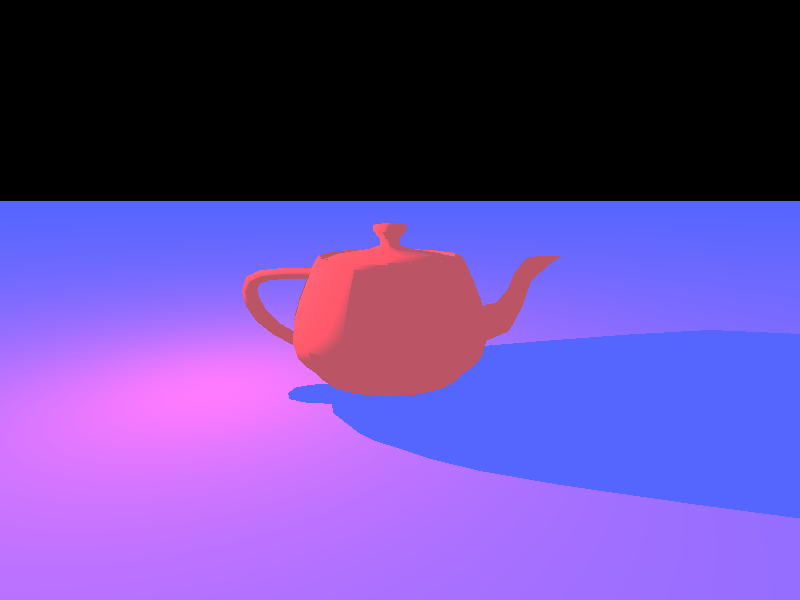
And, to maximize learning, I think its better to do everything yourself from scratch. A crappy teapot which you did from the first principles is full to the brim with knowledge, while a beautiful landscape which you got by following step-by-step instructions is hollow.

And that’s the gist of the post: I’ll try to teach you as little about ray tracing as possible, to give you just enough clues to get some pixels to the screen. To be more poetic, you’ll draw the rest of the proverbial owl.

This is in contrast to Ray Tracing in One Weekend which does a splendid job teaching ray tracing, but contains way to many spoilers if you want to learn software architecture (rather than graphics programming). In particular, it contains snippets of code. We won’t see that here — as a corollary, all the code you’ll write is fully your invention!

Sadly, there’s one caveat to the plan: as the fundamental task is tracing a ray as it gets reflected through the 3D scene, we’ll need a hefty amount of math. Not an insurmountable amount — everything is going to be pretty visual and logical. But still, we’ll need some of the more advanced stuff, such as vectors and cross product.

If you are very comfortable with that, you can approach the math parts the same way as the programming parts — grab a pencil and a stack of paper and try to work out formulas yourself. If solving math puzzlers is not your cup of tea, feel absolutely free to just look up formulas online. https://avikdas.com/build-your-own-raytracer is a great resource for that. If, however, linear algebra is your worst nightmare, you might want to look for a more step-by-step tutorial (or maybe pick a different problem altogether! Another good exercise is a small chat server, for example).

Algorithm Overview

So, what exactly is ray tracing? Imagine a 3D scene with different kinds of objects: an infinite plane, a sphere, a bunch of small triangles which resemble a teapot from afar. The scene is illuminated by some distant light source, and so objects cast shadows and reflect each other. We observe the scene from a particular view point. Roughly, a ray of light is emitted by a light source, bounces off scene objects and eventually, if it gets into our eye, we perceive a sensation of color, which is mixed from light’s original color, as well the colors of all the objects the ray reflected from.

Now, we are going to crudely simplify the picture. Rather than casting rays from the light source, we’ll cast rays from the point of view. Whatever is intersected by the ray will be painted as a pixels in the resulting image.

Let’s do this step-by-step

Images

The ultimate result of our ray tracer is an image. A straightforward way to represent an image is to use a 2D grid of pixels, where each pixel is an “red, green, blue” triple where color values vary from 0 to 255. How do we display the image? One can reach out for graphics libraries like OpenGL, or image formats like BMP or PNG.

But, in the spirit of simplifying the problem so that we can do everything ourselves, we will simplify the problem! As a first step, we’ll display image as text in the terminal. That is, we’ll print . for “white” pixels and x for “black” pixels.

So, as the very first step, let’s write some code to display such image by just printing it. A good example image would be 64 by 48 pixels wide, with 5 pixel large circle in the center. And here’s the first encounter of math: to do this, we want to iterate all (x, y) pixels and fill them if they are inside the circle. It’s useful to recall equation for circle at the origin: x^2 + y^2 = r^2 where r is the radius.

🎉 we got hello-world working! Now, let’s go for more image-y images. We can roll our own “real” format like BMP (I think that one is comparatively simple), but there’s a cheat code here. There are text-based image formats! In particular, PPM is the one especially convenient. Wikipedia Article should be enough to write our own impl. I suggest using P3 variation, but P6 is also nice if you want something less offensively inefficient.

So, rewrite your image outputting code to produce a .ppm file, and also make sure that you have an image viewer that can actually display it. Spend some time viewing your circle in its colorful glory (can you color it with a gradient?).

If you made it this far, I think you understand the spirit of the exercise — you’ve just implemented an encoder for a real image format, using nothing but a Wikipedia article. It might not be the fastest encoder out there, but it’s the thing you did yourself. You probably want to encapsulate it in a module or something, and do a nice API over it. Go for it! Experiment with various abstractions in the language.

$ my-ray-tracer > image.ppm

One Giant Leap Into 3D

Now that we can display stuff, let’s do an absolutely basic ray tracer. We’ll use a very simple scene: just a single sphere with the camera looking directly at it. And we’ll use a trivial ray tracing algorithm: shoot the ray from the camera, if it hit the sphere, paint black, else, paint white. If you do this as a mental experiment, you’ll realize that the end result is going to be exactly what we’ve got so far: a picture with a circle in it. Except now, it’s going to be in 3D!

This is going to be the most annoying part, as there are a lot of fiddly details to get this right, while the result is, ahem, underwhelming. Let’s do this though.

First, the sphere. For simplicity, let’s assume that its center is at the origin, and it has radius 5, and so it’s equation is

x^2 + y^2 + z^2 = 25

Or, in vector form:

v̅ ⋅ v̅ = 25

Here, v̅ is a point on a sphere (an (x, y, z) vector) and ⋅ is the dot product. As a bit of foreshadowing, if you are brave enough to take a stab at deriving various formulas, keeping to vector notation might be simpler.

Now, let’s place the camera. It is convenient to orient axes such that Y points up, X points to the right, and Z points at the viewer (ie, Z is depth). So let’s say that camera is at (0, 0, -20) and it looks at (0, 0, 0) (so, directly at the sphere’s center).

Now, the fiddly bit. It’s somewhat obvious how to cast a ray from the camera. If camera’s position is C̅, and we cast the ray in the direction d̅, then the equation of points on the ray is

C̅ + t d̅

where t is a scalar parameter. Or, in the cartesian form,

(0 + t dx, 0 + t dy, -20 + t dz)

where (dx, dy, dz) is the direction vector for a particular ray. For example, for a ray which goes straight to the center of the sphere, that would be (0, 0, 1).

What is not obvious is how do we pick direction d? We’ll figure that out later. For now, assume that we have some magical box, which, given (x, y) position of the pixel in the image, gives us the (dx, dy, dz) of the corresponding ray. With that, we can use the following algorithm:

Iterate through all (x, y) pixels of our 64x48 the image. From the (x, y) of each pixel, compute the corresponding ray’s (dx, dy, dz). Check if the ray intersects the sphere. If it does, plaint the (x, y) pixel black.

To check for intersection, we can plug the ray equation, C̅ + t d̅, into the sphere equation, v̅ ⋅ v̅ = r^2. That is, we can substitute C̅ + t d̅ for v̅. As C̅, d̅ and r are specific numbers, the resulting equation would have only a single variable, t, and we could solve for that. For details, either apply pencil and paper, or look up “ray sphere intersection”.

But how do we find d̅ for each pixel? To do that, we actually need to add the screen to the scene. Our image is 64x48 rectangle. So let’s place that between the camera and the sphere.

We have camera at (0, 0, -20) our rectangular screen at, say, (0, 0, -10) and a sphere at (0, 0, 0). Now, each pixel in our 2D image has a corresponding point in our 3D scene, and we’ll cast the ray from camera’s position through this point.

The full list of parameters to define the scene is:

sphere center:   0 0 0
sphere radius:   5
camera position: 0 0 -20
camera up:       0 1 0
camera right:    1 0 0
focal distance:  10
screen width:    64
screen height:   48

Focal distance is the distance from the camera to the screen. If we know the direction camera is looking along and the focal distance, we can calculate the position of the center of the screen, but that’s not enough. The screen can rotate, as we didn’t fixed which side is up, so we need an extra parameter for that. We also add a parameter for direction to the right for convenience, though it’s possible to derive “right” from “up” and “forward” directions.

Given this set of parameters, how do we calculate the ray corresponding to, say, (10, 20) pixel? Well, I’ll leave that up to you, but one hint I’ll give is that you can calculate the middle of the screen (camera position + view direction × focal distance). If you have the middle of the screen, you can get to (x, y) pixel by stepping x steps up (and we know up!) and y steps right (and we know right!). Once we know the coordinates of the point of the screen through which the ray shoots, we can compute ray’s direction as the difference between that point and camera’s origin.

Again, this is super fiddly and frustrating! My suggestion would be:

• Draw some illustrations to understand relation between camera, screen, sphere, and rays.

• Try to write the code which, given (x, y) position of the pixel in the image, gives (dx, dy, dz) coordinates of the direction of the ray from the camera through the pixel.

• If that doesn’t work, lookup the solution, https://avikdas.com/build-your-own-raytracer/01-casting-rays/project.html describes one way to do it!

Coding wise, we obviously want to introduce some machinery here. The basic unit we need is a 3D vector — a triple of three real numbers (x, y, z). It should support all the expected operations — addition, subtraction, multiplication by scalar, dot product, etc. If your language supports operator overloading, you might look that up know. Is it a good idea to overload operator for dot product? You won’t know unless you try!

We also need something to hold the info about sphere, camera and the screen and to do the ray casting.

If everything works, you should get a familiar image of the circle. But it’s now powered by a real ray tracer and its real honest to god 3D, even if it doesn’t look like it! Indeed, with ray casting and ray-sphere intersection code, all the essential aspects are in place, from now on everything else are just bells and whistles.

Second Sphere

Ok, now that we can see one sphere, let’s add the second one. We need to solve two subproblems for this to make sense. First, we need to parameterize our single sphere with the color (so that the second one looks differently, once we add it). Second, we should no longer hard-code (0, 0, 0) as a center of the sphere, and make that a parameter, adjusting the formulas accordingly. This is a good place to debug the code. If you think you move the sphere up, does it actually moves up in the image?

Now, the second sphere can be added with different radius, position and color. The ray casting code now needs to be adjusted to say which sphere intersected the ray. Additionally, it needs to handle the case where the ray intersects both spheres and figure out which one is closer.

With this machinery in hand, we can now create some true 3D scenes. If one sphere is fully in front of the other, that’s just concentric circles. But if the spheres intersect, the picture is somewhat more interesting.

Let There Be Phong

The next step is going to be comparatively easy implementation wise, but it will fill our spheres with vibrant colors and make them spring out in their full 3D glory. We will add light to the scene.

Light source will be parameterized by two values:

• Position of the light source.

• Color and intensity of light.

For the latter, we can use a vector with three components (red, green, blue), where each components varies from 0.0 (no light) to 1.0 (maximally bright light). We can use a similar vector to describe a color of the object. Now, when the light hits the object, the resulting color would be a componentwise product of the light’s color and the object’s color.

Another contributor is the direction of light. If the light falls straight at the object, it seems bright. If the light falls obliquely, it is more dull.

Let’s get more specific:

• P̅ is a point on our sphere where the light falls.

• N̅ is the normal vector at P̅. That is, it’s a vector with length 1, which is locally perpendicular to the surface at P̅

• L̅ is the position of the light source

• R̅ is a vector of length one from P̅ to L̅: R̅ = (L̅ - P̅) / |L̅ - P̅|

Then, R̅ ⋅ N̅ gives us this “is the light falling straight at the surface?” coefficient between 0 and 1. Dot product between two unit vectors measures how similar their direction is (it is 0 for perpendicular vectors, and 1 for collinear ones). So, “is light perpendicular” is the same as “is light collinear with normal” is dot product.

The final color will be the memberwise product of light’s color and sphere’s color multiplied by this attenuating coefficient. Putting it all together:

For each pixel (x, y) we cast a C̅ + t d̅ ray through it. If the ray hits the sphere, we calculate point P where it happens, as well as sphere’s normal at point P. For sphere, normal is a vector which connects sphere’s center with P. Then we cast a ray from P to the light source L̅. If this ray hits the other sphere, the point is occluded and the pixel remains dark. Otherwise, we compute the color using using the angle between normal and direction to the light.

With this logic in place, the picture now should display two 3D-looking spheres, rather than a pair of circles. In particular, our spheres now cast shadows!

What we implemented here is a part of Phong reflection model, specifically, the diffuse part. Extending the code to include ambient and specular parts is a good way to get some nicer looking pictures!

Scene Description Language

At this point, we accumulated quite a few parameters: camera config, positions of spheres, there colors, light sources (you totally can have many of them!). Specifying all those things as constants in the code makes experimentation hard, so a next logical step is to devise some kind of textual format which describes the scene. That way, our ray tracer reads a textual screen description as an input, and renders a .ppm as an output.

One obvious choice is to use JSON, though it’s not too convenient to edit by hand, and bringing in a JSON parser is contrary to our “do it yourself” approach. So I would suggest to design your own small language to specify the scene. You might want to take a look at https://kdl.dev for the inspiration.

Note how the program grows bigger — there are now distinctive parts for input parsing, output formatting, rendering per-se, as well as the underlying nascent 3D geometry library. As usual, if you feel like organizing all that somewhat better, go for it!

Plane And Other Shapes

So far, we’ve only rendered spheres. There’s a huge variety of other shapes we can add, and it makes sense to tackle at least a couple. A good candidate is a plane. To specify a plane, we need a normal, and a point on a plane. For example, N̅ ⋅ v̅ = 0 is the equation of the plain which goes through the origin and is orthogonal to N̅. We can plug our ray equation instead of v̅ and solve for t as usual.

The second shape to add is a triangle. A triangle can be naturally specified using its three vertexes. One of the more advanced math exercises would be to derive a formula for ray-triangle intersection. As usual, math isn’t the point of the exercise, so feel free to just look that up!

With spheres, planes and triangles which are all shapes, there clearly is some amount of polymorphism going on! You might want to play with various ways to best express that in your language of choice!

Meshes

Triangles are interesting, because there are a lot of existing 3D models specified as a bunch of triangles. If you download such a model and put it into the scene, you can render somewhat impressive images.

There are many formats for storing 3D meshes, but for out purposes .obj files are the best. Again, this is a plain text format which you can parse by hand.

There are plenty of .obj models to download, with the Utah teapot being the most famous one.

Note that the model specifies three parameters for each triangle’s vertex:

• coordinate (v)

• normal (vn)

• texture (vt)

For the first implementation, you’d want to ignore vn and vt, and aim at getting a highly polygonal teapot on the screen. Note that the model contains thousands of triangles, and would take significantly more time to render. You might want to downscale the resolution a bit until we start optimizing performance.

To make the picture less polygony, you’d want to look at those vn normals. The idea here is that, instead of using a true triangle’s normal when calculating light, to use a fake normal as if the the triangle wasn’t actually flat. To do that, the .obj files specifies “fake” normals for each vertex of a triangle. If a ray intersects a triangle somewhere in the middle, you can compute a fake normal at that point by taking a weighted average of the three normals at the vertexes.

At this point, you should get a picture roughly comparable to the one at the start of the article!

Performance Optimizations

With all bells and whistles, our ray tracer should be rather slow, especially for larger images. There are three tricks I suggest to make it faster (and also to learn a bunch of stuff).

First, ray tracing is an embarrassingly parallel task: each pixel is independent from the others. So, as a quick win, make sure that you program uses all the cores for rendering. Did you manage to get a linear speedup?

Second, its a good opportunity to look into profiling tools. Can you figure out what specifically is the slowest part? Can you make it faster?

Third, our implementation which loops over each shape to find the closest intersection is a bit naive. It would be cool if we had something like a binary search tree, which would show us the closest shape automatically. As far as I know, there isn’t a general algorithmically optimal index data structure for doing spatial lookups. However, there’s a bunch of somewhat heuristic data structures which tend to work well in practice.

One that I suggest implementing is the bounding volume hierarchy. The crux of the idea is that we can take a bunch of triangles and place them inside a bigger object (eg, a gigantic sphere). Then, if a ray doesn’t intersect this bigger object, we don’t need to check any triangles contained within. There’s a certain freedom in how one picks such bounding objects.

For BVH, we will use axis-aligned bounding box as our bounding volumes. It is a cuboid whose edges are parallel to the coordinate axis. You can parametrize an AABB with two points — the one with the lowest coordinates, and the one with the highest. It’s also easy to construct an AABB which bounds a set of shapes — take the minimum and maximum coordinates of all vertexes. Similarly, intersecting an AABB with a ray is fast.

The next idea is to define a hierarchy of AABBs. First, we define a root AABB for the whole scene. If the ray doesn’t hit it, we are done. The root box is then subdivided into two smaller boxes. The ray can hit one or two of them, and we recur into each box that got hit. Worst case, we are recurring into both subdivisions, which isn’t any faster, but in the common case we can skip at least a half. For simplicity, we also start with computing an AABB for each triangle we have in a scene, so we can think uniformly about a bunch of AABBs.

Putting everything together, we start with a bunch of small AABBs for our primitives. As a first step, we compute their common AABB. This will be the basis of our recursion step: a bunch of small AABBs, and a huge AABB encompassing all of them. We want to subdivide the big box. To do that, we select its longest axis (eg, if the big box is very tall, we aim to cut it in two horizontally), and find a midpoint. Then, we sort small AABBs into those whoche center is before or after midpoint along this axis. Finally, for each of the two subsets we compute a pair of new AABBs, and then recur.

Crucially, the two new bounding boxes might intersect. We can’t just cut the root box in two and unambiguously assign small AABBs to the two half, as they might not be entirely within one. But, we can expect the intersection to be pretty small in practice.

Next Steps

If you’ve made it this far, you have a pretty amazing pice of software! While it probably clocks at only a couple of thousands lines of code, it covers a pretty broad range of topics, from text file parsing to advanced data structures for spatial data. I deliberately spend no time explaining how to best fit all these pieces into a single box, that’s the main thing for you to experiment with and to learn.

There are two paths one can take from here:

• If you liked the graphics programming aspect of the exercise, there’s a lot you can do to improve the quality of the output. https://pbrt.org is the canonical book on the topic.

• If you liked the software engineering side of the project, you can try to re-implement it in different programming languages, to get a specific benchmark to compare different programming paradigms. Alternatively, you might want to look for other similar self-contained hand-made projects. Some options include:

  • Software rasterizer: rather than simulating a path of a ray, we can project triangles onto the screen. This is potentially much faster, and should allow for real-time rendering.

  • A highly concurrent chat server: a program which listens on a TCP port, allows clients to connect to it and exchange messages.

  • A toy programming language: going full road from a text file to executable .wasm. Bonus points if you also do an LSP server for your language.

  • A distributed key-value store based on Paxos or Raft.

  • A toy relational database