In a previous article I discussed the situation where you have a sequence of (x,y) points and you want to find the area under the curve that is defined by those points. I pointed out that usually you need to use statistical modeling before it makes sense to compute the area.

However, there is a numerical technique that is very useful for a wide range of numerical integration scenarios, and that is the trapezoidal rule.

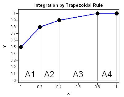
The following graph illustrates the trapezoidal rule. Given a set of points (x1, y1), (x2, y2), ..., (xn, yn), with x1 ≤ x2 ≤ ... ≤ xn, the trapezoidal rule computes the area of the piecewise linear curve that passes through the points. You can compute the area under the piecewise linear segments by summing the area of the trapezoids A1, A2, A3, and A4. (Sometimes a trapezoid is degenerate and is actually a rectangle or a triangle.)

Implementing the Trapezoidal Rule in SAS/IML Software

It is easy to use SAS/IML software (or the SAS DATA step) to implement the trapezoidal rule. The area of a trapezoid defined by (xi, yi) and (xi+1, yi+1) is

( xi+1 – xi ) ( yi + yi+1 ) / 2

The first term is just the width of the subinterval [xi, xi+1] and the second term is the average of the heights at each end of the subinterval.

The following user-defined function computes the area under the piecewise linear segments that connect the points. The function does not check that the x values are sorted in nondecreasing order.

proc iml;
/**Given two vectors x,y where y=f(x), this module
   approximates the definite integral int_a^b f(x) dx 
   by the trapezoid rule. 
   The vector x is assumed to be in numerically increasing
   order so that a=x[1] and b=x[nrow(x)].
   The module does not assume equally spaced intervals.
   The formula is 
   Integral = Sum(  (x[i+1] - x[i]) * (y[i] + y[i+1])/2 )   
**/
start TrapIntegral(x,y);
   N = nrow(x);
   dx    =   x[2:N] - x[1:N-1];
   meanY = ( y[2:N] + y[1:N-1] )/2;
   return( dx` * meanY );
finish;
 
/** test it **/
x = {0.0, 0.2, 0.4, 0.8, 1.0};
y = {0.5, 0.8, 0.9, 1.0, 1.0};
area = TrapIntegral(x,y);
print area;

Notice that the implementation does not require equally spaced points. The width of all subintervals are computed in a single statement and assigned to the vector dx. Similarly, the average of the heights are computed in a single statement and assigned to the vector meanY. The summation of all the areas is then computed by using a dot product of vectors. (Equivalently, the module could also return the quantity sum(dx # meanY), but the dot product is the more efficient computation.)

The simplicity of the trapezoidal rule makes it an ideal for many numerical integration tasks. Also, the trapezoidal rule is exact for piecewise linear curves such as an ROC curve. Also, as John D. Cook points out, there are other situations in which the trapezoidal rule performs more accurately than other, fancier, integration techniques.

The trapezoidal rule is not as accurate as Simpson's Rule when the underlying function is smooth, because Simpson's rule uses quadratic approximations instead of linear approximations. The formula is usually given in the case of an odd number of equally spaced points. Leave a comment to discuss the relative advantages and disadvantages of Simpson's rule as compared to the trapezoidal rule.

In a future blog post, I will use the TrapIntegral function to integrate some functions that arise in statistical data analysis.