

Bringing WRF up to speed with Arm Neoverse
source link: https://community.arm.com/arm-community-blogs/b/high-performance-computing-blog/posts/bringing-wrf-up-to-speed-with-arm-neoverse
Go to the source link to view the article. You can view the picture content, updated content and better typesetting reading experience. If the link is broken, please click the button below to view the snapshot at that time.

Background
The better understanding of climate change and more reliable weather forecasting requires sophisticated numerical weather prediction models which consume large amounts of High Performance Computing (HPC) resources. Interest in cloud-based HPC for such models continues to grow [1].
One such widely used application is the WRF (Weather Research and Forecasting) model. This blog discusses running a simple WRF model on the AWS Graviton2 and AWS Graviton3 processors, which are both based on Arm Neoverse core designs. Interestingly, the AWS Graviton3 is the first cloud-based processor that has the Arm Scalable Vector Extension (SVE) ISA and DDR5 memory. We look at the performance of WRF on both instance types and review a few easy steps to consider to maximize performance.
Instances
The AWS Graviton2 (c6g) was introduced back in 2019 and is based on the Arm Neoverse N1 core design. Each N1 core operates with 2x128-bit (Neon) floating-point units per cycle. The AWS Graviton3 (c7g) was introduced back in late 2021 and is based on the Arm Neoverse V1 core design. Neoverse V1 also has SVE which enables wider vectors than with Neon. The AWS Graviton3 has a vector width of 256-bits, meaning it can operate with either 2x256-bit (SVE) or 4x128-bit (Neon) floating-point units per cycle. So in theory a 2x increase in floating-point performance is possible.
|
Instance |
Amazon Linux 2 kernel |
CPU |
Memory |
|
c6g.16xlarge |
4.14.294-220.533.amzn2.aarch64 |
64xAWS Graviton2 single socket. Running at 2.5GHz |
8 memory channels of DD4-3200 Single NUMA regions |
|
c7g.16xlarge |
5.10.144-127.601.amzn2.aarch64 |
64xAWS Graviton3 single socket. Running at 2.6GHz |
8 memory channels of DD5-4800 Single NUMA regions |
In terms of multi-node capability the c6g(n) is AWS 100Gbs EFA ready, whereas the c7g is currently only available with a 30Gbs network. For WRF, there are two well-known test cases: Conus12km which can be run on a single node, and the larger Conus2.5km, which is more suited to multi-node runs. Here, we keep to single node Conus12km runs, to keep the discussion around features in common between instances. In practice, the impact of the speed of the interconnect on scalability depends on the size of the WRF case of interest and how many instances used. For some cases, this might be around 16+ instances [2].
Build details
We use WRF4.4, which is the current release, along with dependencies: OpenMPI-4.1.3, HDF5-1.13.1, NetCDF-C-4.8.1 and NetCDF-F-4.5.4. These dependencies are built with GCC-12.2.0 across all AWS instances. It is equally possible to use other toolchains to build WRF, such as the Arm Compiler for Linux or the NVIDIA HPC Software Development Kit (SDK) [3]. GCC currently just has a small edge on out-of-the-box performance for this particular test. The flags used are shown in the following table.
| Instance | GCC12.2.0 flags |
| c6g | -march=armv8.2-a -mtune=neoverse-n1 |
| c7g | -march=armv8.4-a -mtune=neoverse-512tvb |
The dependencies build without any modification across all selected instances, however WRF4.4 itself does need a few minor modifications. These modifications can be applied at the configuration step, as mentioned here. If for any reason a build fails, then it is worth checking the configure.wrf file to see that the correct flags are set.
Performance comparison
Performing runs on each instance gives us the following. We found that running with 8 MPI tasks and 8 OpenMP threads per task gave best overall results. Here s/ts denotes seconds/time step (or Mean Time per Step) and is taken as the average of the values for 'Timing for main' from the resulting rsl.error.0000 file.
|
Instance |
s/ts |
Launch line (OMP_NUM_THREADS=8 OMP_PLACES=cores) |
|
c6g.16xlarge |
1.6383 |
mpirun -n 8 --report-bindings --map-by socket:PE=8 ./wrf.exe |
|
c7g.16xlarge |
1.13068 |
mpirun -n 8 --report-bindings --map-by socket:PE=8 ./wrf.exe |
Let us consider c6g vs c7g performance, as there is a significant difference. What is helping the most on the c7g? Is it having double the vector width, SVE instructions, or the faster DDR5 memory? Checking whether it is the SVE instructions is easy, just by running the c6g (AWS Graviton2) built (non-SVE) executable on the c7g. In fact, we see that performance is almost the same, telling us that it is not the SVE helping here. So, the uplift is mostly from the faster memory bandwidth with DDR5 and the 4x128-bit (Neon) floating-point units.
It is worth mentioning that checking SVE vs Neon performance for your application is a good idea on any SVE enabled processor. It really depends on the application whether it is able to utilize SVE instructions optimally.
Better performance without effort
If we have a closer look at the performance, using Arm Forge we can see that the c6g shows 0.98 Cycles Per Instruction, whereas c7g is much lower at 0.66 (same for Neon or SVE). This reduction is also contributing to the performance uplift going from c6g to c7g and is due to the improved Neoverse V1 CPU pipeline. It is also worth noting that the overall wall-clock times for c6g and c7g are 896s and 614s, respectively. Can we do anything to lower these times?
From the list of Functions in Figure 1 we see that powf_finite, which is from the standard C library of basic mathematical functions(libm-2.26), is taking 6.1% of the overall runtime. There are also other similar functions taking around 1% of this time, along with memset and memcpy from the standard C library (libc-2.26).
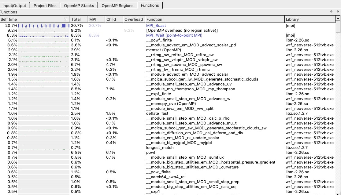
Figure 1: List of top functions
We can improve on this result very easily by replacing the implementation of these functions with ones from the Arm Performance Libraries. This library not only contains highly optimized routines for BLAS, LAPACK, and FFTW but also libamath, which has the widely used functions from libm. The library also contains an optimized memset and memcpy in libastring. We can use these libraries by just relinking the main wrf.exe with libamath and libastring (taking care to place the link leftmost to the one for libm), for example.
mpif90 -o wrf.exe … -L/opt/arm/armpl-22.1.0_AArch64_RHEL-7_gcc_aarch64-linux/lib -lastring -L/opt/arm/armpl-22.1.0_AArch64_RHEL-7_gcc_aarch64-linux/lib -lamath -lm -lz
In terms of overall wall-clock time, we measure 821s for c6g and 569s c7g. This is a good improvement for simply switching to another library. Similarly, as recommended here, some applications can benefit from zlib-cloudflare which has been optimized for faster compression. Trying again, this time with the optimized libz, wall-clock times reduce to 776s and 539s for c6g and c7g, respectively. In summary, the corresponding Mean Time per Step values as shown in Figure 2, agree with the overall wall-clock times.
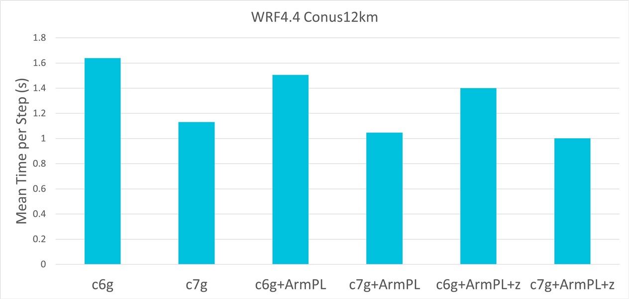
Figure 2: Comparison of Mean Time per Step (s) for c6g and c7g
Summary
In this blog we have taken a widely used numerical weather prediction model, WRF4.4, and compared performance for two AWS EC2 instances: the AWS Graviton2 (c6g) and AWS Graviton3 (c7g). For a standard GCC12.2.0 build of WRF4.4 we have seen that the c7g gives 30% better performance than c6g. We have also seen how easy it is to achieve a further 13% performance improvement by using the Arm Performance Libraries and an optimized implementation of zlib.
References
[2] https://aws.amazon.com/blogs/hpc/numerical-weather-prediction-on-aws-graviton2/
[3] https://github.com/arm-hpc-devkit/nvidia-arm-hpc-devkit-users-guide/blob/main/examples/wrf.md
Recommend
About Joyk
Aggregate valuable and interesting links.
Joyk means Joy of geeK