

The modelling process with neural networks
source link: https://www.neuraldesigner.com/blog/modelling-process
Go to the source link to view the article. You can view the picture content, updated content and better typesetting reading experience. If the link is broken, please click the button below to view the snapshot at that time.

The modelling process with neural networks
Introduction
Neural networks are the most crucial technique for machine learning and artificial intelligence. Mathematically, we can formulate the modelling process with neural networks from a variational point of view. Indeed, building a model consists of finding a function that causes some functional to assume an extreme value.
The following figure depicts an class diagram for the concepts involved in the modelling process.
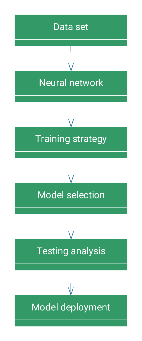
As we can see, the modelling process involves six concepts: data set, neural network, training strategy, model selection, testing analysis, and model deployment. Next, we introduce these six concepts.
1. Data set
The data set contains information for creating our model.The information may include numerical measurements, text, images, etc. It is a data collection structured as a table in rows and columns.
A data set comprises a matrix and information about the columns or variables and rows or samples. Variables can be used as inputs, targets, or unused. Samples can be used for training, selection, testing, or unused.
The following is an example of an data set in the automotive sector.
Example: Electric motor data set
An automotive company wants to build a digital twin of an electric motor using artificial intelligence. Having robust estimators of rotor and stator temperature helps the automotive industry to improve the motor's efficiency by reducing power losses and, ultimately, heat buildup.
The company uses the data set to build the model. The dataset comprises various sensor data collected from a permanent magnet synchronous motor (PMSM) deployed on a test bench. The testbed measurements were collected by the LEA department of the University of Paderborn. This data set consists of 107 samples.
The following table illustrates the data set.
| ambient temperature | coolant temperature | voltage_d | voltage_q | ... | stator_winding |
|---|---|---|---|---|---|
| -0.274 | -1.070 | 0.180 | 1.681 | ... | -0.331 |
| -0.274 | -1.070 | -1.243 | 0.483 | ... | 0.712 |
| -0.274 | -1.070 | -1.560 | -0.504 | ... | 1.519 |
| -0.274 | -1.070 | 0.298 | 0.958 | ... | -1.767 |
| -0.274 | -1.070 | -0.963 | 0.642 | ... | -0.846 |
| -0.274 | -1.070 | -1.498 | -0.140 | ... | -0.947 |
| -0.274 | -1.070 | -1.026 | 0.926 | ... | -0.346 |
| ... | ... | ... | ... | ... | ... |
| -0.127 | 1.930 | 0.300 | -1.292 | ... | 0.372 |
In this data set, all the variables are numeric. The input variables are ambient_temperatureambient_temperature, coolant_temperaturecoolant_temperature, voltage_dvoltage_d, voltage_qvoltage_q, voltage_modulevoltage_module, current_dcurrent_d, current_qcurrent_q and current_modulecurrent_module and the target variables are motor_speedmotor_speed, torquetorque, stator_yokestator_yoke and stator_toothstator_tooth, stator_windingstator_winding.
The samples are divided into 60% training samples (65), 20% selection samples (21) and the remaining 20% in testing samples (21).
2. Neural network
An artificial neural network, or simply a neural network, can be defined as a biologically inspired computational algorithm consisting of a network architecture composed of artificial neurons.
This structure contains a set of parameters tuned to perform specific tasks. The neural network represents the model.
Neural networks are organised in layers. Approximation models typically contain two layers of perceptronperceptron. Classification models usually contain a perceptronperceptron layer and a probabilisticprobabilistic layer. Forecasting models usually contain a recurrent layer and a perceptronperceptron layer. Other models, such as the image classification model, include multiplate convolutionalconvolutional and pullingpulling layers and a perceptronperceptron or probabilisticprobabilistic layer.
Neural networks have universal approximation properties. This means that they can approximate any function in any dimension with a desired degree of accuracy.
The following is an example of neural network in the automotive sector.
Example: Electric motor neural network
To create its model, the company chooses a neural network. The following figure shows the neural network model.
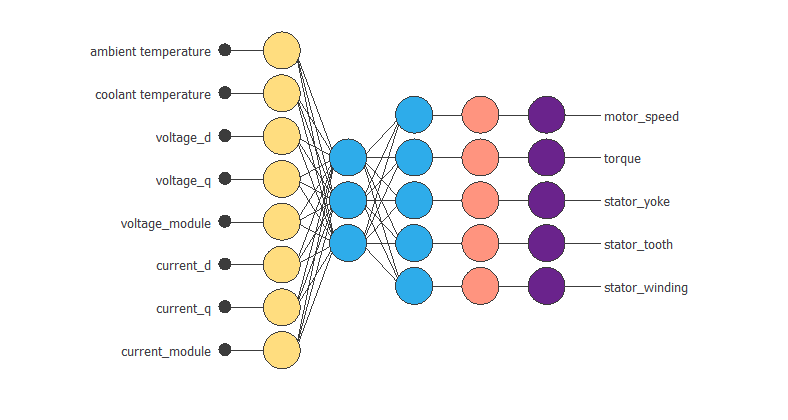
The neural network consists of five layers. The first is a scaling layer with eight neurons; the two followings are perceptron layers with three and five neurons, respectively, and the last is a probabilistic layer with five neurons.
As we can see, the inputs to this neural network are ambient_temperatureambient_temperature, coolantcoolant, voltage_dvoltage_d, voltage_qvoltage_q, current_dcurrent_d, current_qcurrent_q, voltage_modulevoltage_module and current_modulecurrent_module. The outputs from the neural network are motor_speedmotor_speed, torquetorque, stator_yokestator_yoke, stator_toothstator_tooth and stator_windingstator_winding.
3. Training strategy
The objective of the training strategy is to fit the data set to the neural network. The training strategy comprises the loss index and the optimisation algorithm.
The loss index defines the task the neural network is required to do and provides a measure of the quality of the representation that the model is necessary to learn. The choice of a suitable error term depends on the particular application. We can state the learning problem to minimise the loss index
The loss index for a neural network is composed of terms. The more important are the error term and the regularisation term. The error term measures the difference between the outputs of the neural network and the correct predictions.
We can use several types of errors. The most common error functions are Mean Squared ErrorMeanSquaredError, Normalised Squared ErrorNormalisedSquaredError, Minkowski ErrorMinkowskiError, Cross−Entropy ErrorCross−EntropyError in classification problems or the Squared Weighted ErrorSquaredWeightedError in binary classification problems.
The regularisation term can be applied to obtain a good generalisation. Adding a regularisation term to the error term will decrease the values of the biases and the neural network's weights. In consequence, the outputs of the neural network will become smoother, avoiding overfitting. One of the most used regularisation methods is the norm of the neural network parameters.
The primary purpose of the loss index is to avoid overfitting and improve regularisation. Among the most commonly used optimisation algorithms are Gradient DescentGradientDescent, Conjugate GradientConjugateGradient, Quasi−Newton MethodQuasi−NewtonMethod, Levenberg−MarquardtLevenberg−Marquardt, Stochastic Gradient DescentStochasticGradientDescent and Adaptative Moment EsrimationAdaptativeMomentEsrimation.
The following is an example of a training strategy in the automotive sector.
Example: Electric motor training strategy
An automotive company creates a model to improve the efficiency of its engines. The loss index chosen is the normalised squared error with L2 regularisation. This loss index is the default in approximation applications. The optimisation algorithm chosen is the quasi-Newton method. Once the strategy has been set, we can train the neural network.
The following figure shows how the training (blue) and selection (orange) errors decrease with the training epoch during the training process.
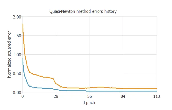
The chart shows that both errors decrease until reaching a stationary value, so the algorithm converges. The most critical training result is the final selection error. It is a measure of the generalisation ability of the neural network. The final selection error and training error are selection error=0.083NSEselectionerror=0.083NSE and training error=0.029NSEtrainingerror=0.029NSE.
4. Model selection
As we said before, building a model's objective is not to memorise the training subset but to show a good generalisation capacity. The optimal architecture is the one that shows the best generalisation capacity. That is the one for which the selection error is the lowest. We can analyse which input variables are redundant and deleted from the neural network, called inputs selection. It can be studied for which number of neurons the neural network shows the best performance, called neuron selection.
When designing the neural network architecture, two common problems can occur: underfitting and overfitting.
Underfitting is the effect that appears when the model is too simple. In this case, the neural network can fit neither the training data nor the selection data. Overfitting is the opposite effect. It occurs when the neural network is too complex. Consequently, during the training process, the error for the training samples will decrease while the error for the selected samples increases. In both situations, the result is a model of bad quality.
The following is an example of a model selection in the automotive sector.
Example: Electric motor model selection
To achieve the model's optimal architecture, the company studies which input variables are redundant and with which number of neurons the neural network shows the best performance. This reduces the selection error in its model. They use the growing neuron algorithm to achieve the optimal number of neurons.
The following figure shows the final neural network model.
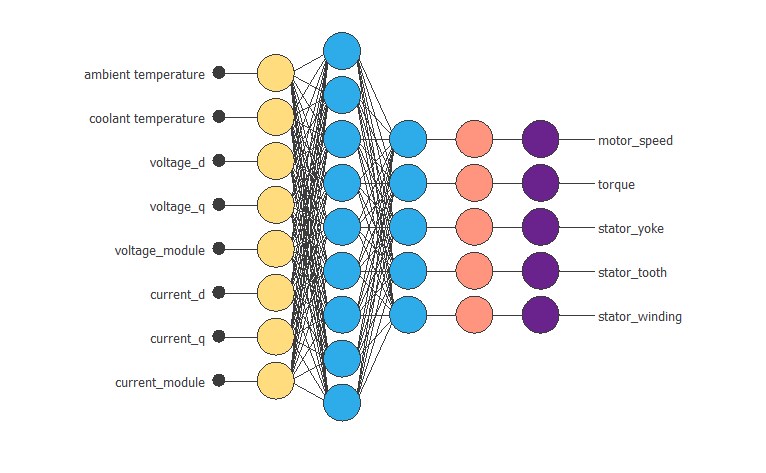
Therefore, the number of neurons in the perceptron layer has increased from 3 to 9 and the selection error has changed from 0.083NSE0.083NSE to 0.043NSE0.043NSE.
5. Testing analysis
Once the optimisation algorithm has trained the model, we must evaluate its predictive ability on new data previously seen in the neural network.
We use the test subset, which contains a set of new cases with their corresponding inputs and target variables. The goal of testing is to compare the responses of the trained neural network with the correct predictions for each sample in the test subset.
We can use the results of this process as a simulation of what would happen in a real-world situation.
One of the simplest methods to study the neural network's performance is calculating the error for the testing subset. If the model has not over-fitted the training or selection instances, the training, selection, and testing errors should be similar.
The most common method for testing regression models is the goodness of fit analysis. In the case of classification, the confusion matrix, the binary classification tests, or the ROC curve are quite common testing methods. There are also specific methods for testing forecasting models. Some of them are error autocorrelations and inputs-error cross-correlations.
If we consider the neural network good quality, we can move it to the deployment phase.
The following is an example of a testing analysis in the automotive sector.
Example: Electric motor testing analysis
The automotive company needs to test the model to check how well it fits a set of observations. To do this, they choose to calculate the goodness of fit of a statistical model and the coefficient of determination, R2.
The total number of test samples is 21.
The model's goodness-of-fit measures summarise the discrepancy between observed and expected values. The R2 coefficient quantifies the proportion of variation of the predicted variable concerning the actual values. If we had a perfect fit (results equal to the objectives), R2 would be equal to 1.
The following figure illustrates the predicted values versus the actual ones for the output stator_yokestator_yoke.
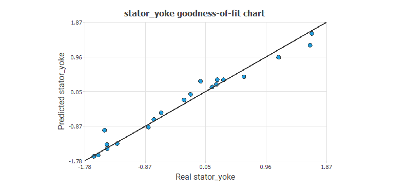
The chart shows that the predicted values resemble the actual values.
To give a quality measure, we calculate the coefficient of determination, R22.
| Value | |
|---|---|
| Determination | 0.970 |
Indeed, the regularisation coefficient R2 is close to 1.
6. Model deployment
The concept of deployment in machine learning refers to applying a model to predict new data.
The deployment of a model consists of making it available to end-users. There are many ways to deploy a machine learning model.
The form of deployment depends on the requirements. Sometimes, the end-user wants a report with the results. On other occasions, they might need a repeatable continuous learning process.
The following is an example of a model deployment in the automotive sector.
Example: Electric motor model deployment
The mathematical function describes the operation of the motor from the input data.
The mathematical expression represented by the neural network is written below.
        scaled_ambient temperature = (ambient temperature+0.6031910181)/0.98526299;
scaled_coolant temperature = (coolant temperature+0.3932940066)/1.030290008;
scaled_voltage_d = (voltage_d+0.3587549925)/0.799169004;
scaled_voltage_q = (voltage_q+0.2354030013)/0.9717490077;
scaled_voltage_module = (voltage_module-1.255239964)/0.4234420061;
scaled_current_d = (current_d-0.08343230188)/1.120489955;
scaled_current_q = (current_q-0.2310259938)/0.6012690067;
scaled_current_module = (current_module-1.189710021)/0.4886389971;

perceptron_layer_1_output_0 = tanh( -0.293822 + (scaled_ambient temperature*0.017537) + (scaled_coolant temperature*0.277449) + (scaled_voltage_d*-0.147449) + (scaled_voltage_q*0.0689801) + (scaled_voltage_module*-0.0169951) + (scaled_current_d*-0.267293) + (scaled_current_q*-0.385712) + (scaled_current_module*0.0363538) );
perceptron_layer_1_output_1 = tanh( -0.00602507 + (scaled_ambient temperature*-0.0122427) + (scaled_coolant temperature*-0.447815) + (scaled_voltage_d*-0.036908) + (scaled_voltage_q*0.00900047) + (scaled_voltage_module*-0.0253258) + (scaled_current_d*0.27237) + (scaled_current_q*-0.163464) + (scaled_current_module*-0.115275) );
perceptron_layer_1_output_2 = tanh( 0.224242 + (scaled_ambient temperature*-0.00884039) + (scaled_coolant temperature*-0.210512) + (scaled_voltage_d*-0.0931465) + (scaled_voltage_q*0.0881369) + (scaled_voltage_module*0.0192406) + (scaled_current_d*-0.0520755) + (scaled_current_q*0.185785) + (scaled_current_module*-0.0117133) );

perceptron_layer_2_output_0 = ( 0.141026 + (perceptron_layer_1_output_0*2.54465) + (perceptron_layer_1_output_1*0.551241) + (perceptron_layer_1_output_2*2.39387) );
perceptron_layer_2_output_1 = ( -0.723429 + (perceptron_layer_1_output_0*-1.79491) + (perceptron_layer_1_output_1*-1.76963) + (perceptron_layer_1_output_2*1.484) );
perceptron_layer_2_output_2 = ( 0.231167 + (perceptron_layer_1_output_0*0.653582) + (perceptron_layer_1_output_1*-1.86523) + (perceptron_layer_1_output_2*-0.536217) );
perceptron_layer_2_output_3 = ( 0.155599 + (perceptron_layer_1_output_0*1.09885) + (perceptron_layer_1_output_1*-1.7018) + (perceptron_layer_1_output_2*0.494817) );
perceptron_layer_2_output_4 = ( 0.0824158 + (perceptron_layer_1_output_0*1.09379) + (perceptron_layer_1_output_1*-1.57303) + (perceptron_layer_1_output_2*1.0116) );

unscaling_layer_output_0=perceptron_layer_2_output_0*1.132040024-0.06418219954;
unscaling_layer_output_1=perceptron_layer_2_output_1*0.604493022+0.2313710004;
unscaling_layer_output_2=perceptron_layer_2_output_2*0.9934260249-0.4365360141;
unscaling_layer_output_3=perceptron_layer_2_output_3*1.083299994-0.401120007;
unscaling_layer_output_4=perceptron_layer_2_output_4*1.152959943-0.3688929975;
The mathematical function is the final result of the study. The company can use it to achieve its objectives: to improve the efficiency of its car engines.
Do you need help? Contact us | FAQ | Privacy | © 2022, Artificial Intelligence Techniques, Ltd.
Recommend
About Joyk
Aggregate valuable and interesting links.
Joyk means Joy of geeK