Plotting Mathematical Functions in Python Part 1

There is a wealth of information out there on plotting mathematical functions in Python, typically using NumPy to create a set of y values for a range of x values and plotting them with Matplotlib. In this article I will write a simple but powerful function to abstract away much of the repetitive code necessary to do this. In future articles I will show the code in use for a selection of functions.

Plotting Mathematical Functions

Functions which map an x value to a corresponding y value are a key part of mathematics, and calculating and plotting y values for a range of x values is a very common task. As a simple example take a look at the graph below which shows the squares of x, more formally known as a quadratic equation and written like this:

y = x2

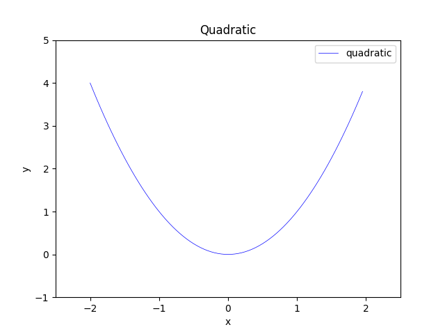
The values of y for this graph were calculated using NumPy and plotted with Matplotlib. The code for doing this is pretty simple but if you need to plot functions regularly it can be repetitive and tedious so just writing the code once in a separate function is very beneficial. It also means of course that any changes need only be made once.

The function I have written for this purpose takes a list of functions to plot as well as a start and end point for the x values. It also takes a number of configuration values which specify the appearance of the graph.

In future articles I will demonstrate the plotting function in use with a selection of different mathematical functions, but in this article I will keep things simple by just plotting the quadratic function shown above.

The Project

This project consists of the following files:

• functionplotter.py
• samplefunctions.py
• functionplotterdemo.py

The files can be downloaded as a zip, or you can clone/download the Github repository if you prefer.

Source Code Links

ZIP File
GitHub

The Function Plotter Code

This is functionplotter.py which contains just one function called plot.

functionplotter.py

import math

import numpy as np
import matplotlib
import matplotlib.pyplot as plt


def plot(functions, start, end, step, config):

"""
    Plots the functions in Matplotlib with
    values of x between start and end with specified step.
    The config dictionary contains various settings
    for the behaviour and appearance of the plot.
    """

# set defaults for missing config values

    config["colors"] = config.get("colors", plt.rcParams['axes.prop_cycle'].by_key()['color'])

config["legend_labels"] = config.get("legend_labels", [*range(1, len(functions) + 1)])

plt.title(config.get("title", "Title"))
    plt.xlabel(config.get("xlabel", "xlabel"))
    plt.ylabel(config.get("ylabel", "ylabel"))
    plt.xlim(config.get("x_limit", (start, end)))

if "y_limit" in config:
        plt.ylim(config["y_limit"])

color_count = len(config["colors"])

# list of values we apply functions to

    xvalues = np.arange(start, end, step)

# iterate functions, applying each to x values and plotting result

    for index, function in enumerate(functions):

yvalues = function(xvalues)

plt.plot(xvalues,
                 yvalues,
                 linewidth = config.get("linewidth", 1),
                 label = config["legend_labels"][index],
                 color = config["colors"][index % color_count])


    plt.legend()

plt.show()

Much of this code is concerned with using the values in the config dictionary or setting defaults for any values which are not present. I'll run through these one at a time.

colors - the Python dictionary has a method named get which returns the values for the specified key if it exists, or the specified default value if not. The first line of code sets config["colors"] to itself if present, or Matplotlib's built-in colors if not. The code to retrieve the latter is:

plt.rcParams['axes.prop_cycle'].by_key()['color']

(Maybe one day I'll take a closer look at rcParams to see what other useful stuff is in there.)

legend_labels is a list of strings to display in the legend alongside the color corresponding to each function being plotted. Ideally they should be meaningful descriptions of the functions but if missing they are simply set to 1, 2, 3 etc.

title, xlabel and ylabel are the string to label the overall graph and its two axes, and are set to default strings if missing.

x_limit is a tuple containing the start and end values of x displayed by the graph, and can be different to the start and end arguments of the plot function if you want to leave a bit of space at the sides. If missing they default to the start and end argument values.

y_limit restricts the values of y shown which can be useful for plotting functions which occasionally shoot up or down to extreme values. Here we only set it if present in the config dictionary. If not set then Matplotlib will just show the entire range of y values.

That's the config values dealt with, but we now need to find out the number of colors are available and stick it in a variable color_count. (Matplotlib's default list currently has 10 colors but we can pass a list of any size.)

Now for the easy bit - calculating and plotting values of y. Firstly we need a NumPy array xvalues across the specified range and with the specified step.

Now we iterate the functions list (remember the plot function can handle any number of mathematical functions) and for each one create a NumPy array yvalues by applying the function to xvalues. Now we can plot xvalues and yvalues, also setting linewidth, label and color. The modulus of index and color_count is used to index the colors list so we cycle through them if there are more functions than colors.

After the loop exits we just need to call legend() and show().

Sample Functions

This is the samplefunctions.py file.

samplefunctions.py

samples = {
            "quadratic": (lambda x: x**2)
          }

It contains a dictionary of functions, or at the moment just one function. Many more to come . . .

The quadratic function is so simple it's easiest to use a lambda but you can use full function definitions if you need something more complex.

Putting Things to Work

Now let's look at functionplotterdemo.py where we can try out the code we have so far.

functionplotterdemo.py

import functionplotter as fp
import samplefunctions as sf


def main():

print("--------------------")
    print("| codedrome.com    |")
    print("| Function Plotter |")
    print("--------------------\n")

plot_samples()


def plot_samples():

fp.plot(functions = [sf.samples["quadratic"]],
            start = -2,
            end = 2,
            step = 0.05,
            config = {"legend_labels": ["quadratic"],
                      "title": "Quadratic",
                      "xlabel": "x",
                      "ylabel": "y",
                      "linewidth": 0.5,
                      "colors": [ "#0000FF" ],
                      "x_limit": (-2.5, 2.5),
                      "y_limit": (-1, 5)
                      })


if __name__ == "__main__":

main()

After a couple of import statements the main function calls plot_samples() which contains a single call to plot. The arguments can be a bit fiddly but those used here can be copied, pasted and edited as necessary.

Now run the code with this command.

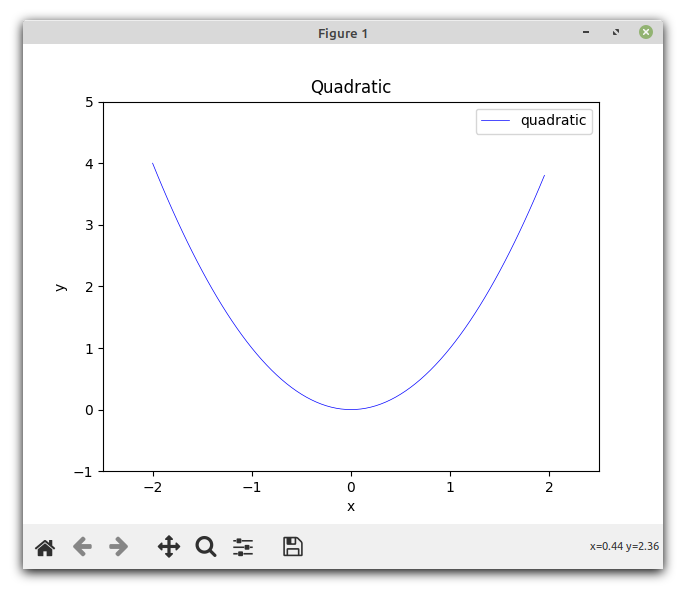
Running the Code

python3 functionplotterdemo.py

This is the result; the graph is the same as shown above but here the Matplotlib window is also shown.

What's Next?

The samples dictionary in samplefunctions.py is miserably sparse at the moment but I have a few further articles planned to plot other functions:

• trigonometric functions such as the familiar sine wave
• more polynomials on top of the quadratic function we have already seen
• derivatives, ie. the gradients or rates of change of a function at each point
• logarithmic and exponential functions
• transformations - moving the curve horizontally and vertically, and stretching it out and squashing it up

For updates on the latest posts please follow CodeDrome on Twitter