

AI 音辨世界:艺术小白的我,靠这个AI模型,速识音乐流派选择音乐 ⛵
source link: https://blog.51cto.com/u_15545802/5624160
Go to the source link to view the article. You can view the picture content, updated content and better typesetting reading experience. If the link is broken, please click the button below to view the snapshot at that time.

AI 音辨世界:艺术小白的我,靠这个AI模型,速识音乐流派选择音乐 ⛵
精选 原创
音乐领域,借助于歌曲相关信息,模型可以根据歌曲的音频和歌词特征,将歌曲精准进行流派分类。本文讲解如何基于机器学习完成对音乐的识别分类。
💡 作者: 韩信子@ ShowMeAI
📘 数据分析实战系列: https://www.showmeai.tech/tutorials/40
📘 机器学习实战系列: https://www.showmeai.tech/tutorials/41
📘 本文地址: https://www.showmeai.tech/article-detail/309
📢 声明:版权所有,转载请联系平台与作者并注明出处
📢 收藏 ShowMeAI查看更多精彩内容

只要给到足够的相关信息,AI模型可以迅速学习一个新的领域问题,并构建起很好的知识和预估系统。比如音乐领域,借助于歌曲相关信息,模型可以根据歌曲的音频和歌词特征将歌曲精准进行流派分类。在本篇内容中 ShowMeAI 就带大家一起来看看,如何基于机器学习完成对音乐的识别分类。
本篇内容使用到的数据集为 🏆 Spotify音乐数据集,大家也可以通过 ShowMeAI 的百度网盘地址快速下载。
🏆 实战数据集下载(百度网盘):公众号『ShowMeAI研究中心』回复『实战』,或者点击 这里 获取本文 [18]音乐流派识别的机器学习系统搭建与调优 『Spotify 音乐数据集』
⭐ ShowMeAI官方GitHub: https://github.com/ShowMeAI-Hub
我们在本篇内容中将用到最常用的 boosting 集成工具库 LightGBM,并且将结合 optuna 工具库对其进行超参数调优,优化模型效果。

关于 LightGBM 的模型原理和使用详细讲解,欢迎大家查阅 ShowMeAI 的文章:
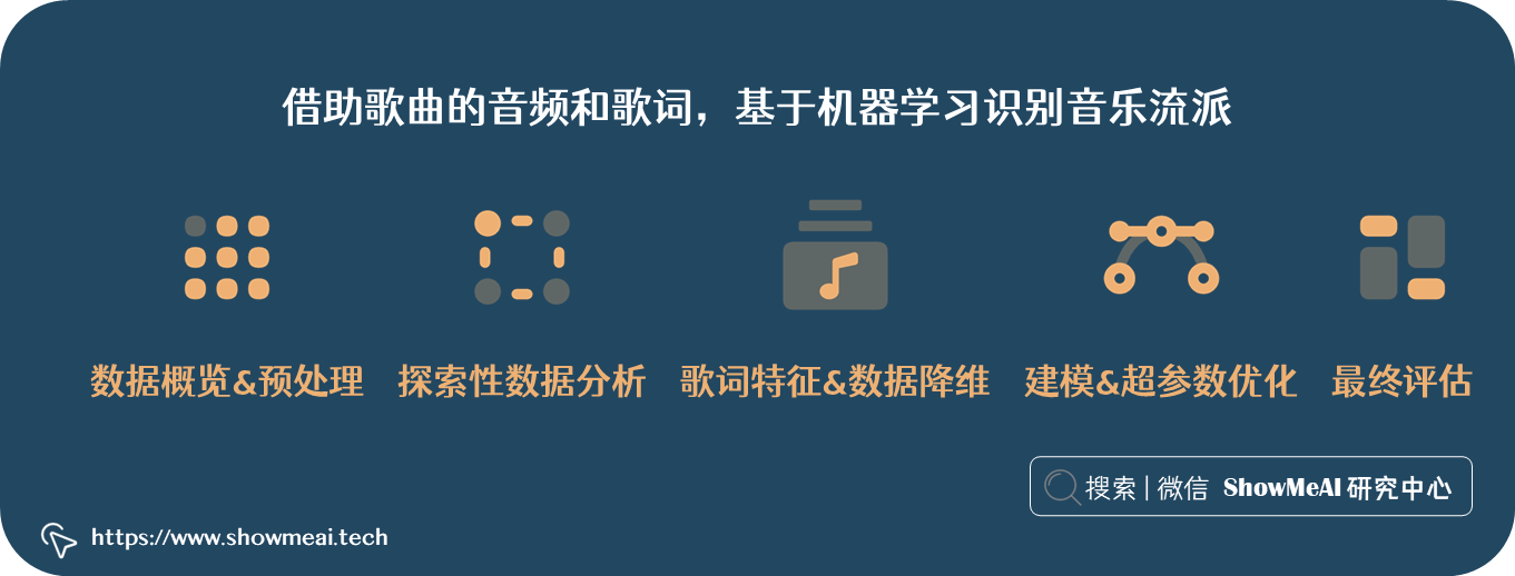
本篇文章包含以下内容板块:
- 数据概览和预处理
- EDA探索性数据分析
- 歌词特征&数据降维
- 建模和超参数优化
- 总结&经验
💡 数据概览和预处理
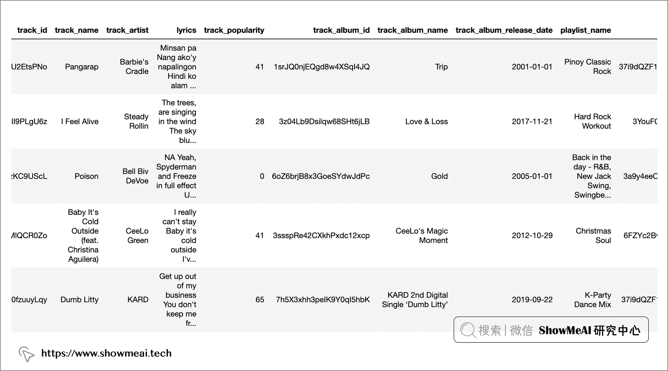
本次使用的数据集包含超过 18000 首歌曲的信息,包括其音频特征信息(如活力度,播放速度或调性等),以及歌曲的歌词。
我们读取数据并做一个速览如下:
import pandas as pd
# 读取数据
data = pd.read_csv("spotify_songs.csv")
# 数据速览
data.head()
# 数据基本信息
data.info()
字段说明如下:
| 字段 | 含义 |
|---|---|
| track_id | 歌曲唯一ID |
| track_name | 歌曲名称 |
| track_artist | 歌手 |
| lyrics | 歌词 |
| track_popularity | 唱片热度 |
| track_album_id | 唱片的唯一ID |
| track_album_name | 唱片名字 |
| track_album_release_date | 唱片发行日期 |
| playlist_name | 歌单名称 |
| playlist_id | 歌单ID |
| playlist_genre | 歌单风格 |
| playlist_subgenre | 歌单子风格 |
| danceability | 舞蹈性描述的是根据音乐元素的组合,包括速度、节奏的稳定性、节拍的强度和整体的规律性,来衡量一首曲目是否适合跳舞。0.0的值是最不适合跳舞的,1.0是最适合跳舞的。 |
| energy | 能量是一个从0.0到1.0的度量,代表强度和活动的感知度。一般来说,有能量的曲目给人的感觉是快速、响亮。例如,死亡金属有很高的能量,而巴赫的前奏曲在该量表中得分较低。 |
| key | 音轨的估测总调。用标准的音阶符号将整数映射为音高。例如,0=C,1=C♯/D♭,2=D,以此类推。如果没有检测到音调,则数值为-1。 |
| loudness | 轨道的整体响度,单位是分贝(dB)。响度值是整个音轨的平均值,对于比较音轨的相对响度非常有用。 |
| mode | 模式表示音轨的调式(大调或小调),即其旋律内容所来自的音阶类型。大调用1表示,小调用0表示。 |
| speechiness | 言语性检测音轨中是否有口语。录音越是完全类似于语音(如脱口秀、说唱、诗歌),属性值就越接近1.0。 |
| acousticness | 衡量音轨是否为声学的信心指数,从0.0到1.0。1.0表示该曲目为原声的高置信度。 |
| instrumentalness | 预测一个音轨是否包含人声。越接近1.0该曲目就越有可能不包含人声内容。 |
| liveness | 检测录音中是否有听众存在。越接近现场演出数值越大。 |
| valence | 0.0到1.0,描述了一个音轨所传达的音乐积极性,接近1的曲目听起来更积极(如快乐、欢快、兴奋),而接近0的曲目听起来更消极(如悲伤、压抑、愤怒)。 |
| tempo | 轨道的整体估计速度,单位是每分钟节拍(BPM)。 |
| duration_ms | 歌曲的持续时间(毫秒) |
| language | 歌词的语言语种 |
原始的数据有点杂乱,我们先进行过滤和数据清洗。
# 数据工具库
import pandas as pd
import re

# 歌词处理的nlp工具库
import nltk
from nltk.corpus import stopwords
from collections import Counter
# nltk.download('stopwords')

# 读取数据
data = pd.read_csv("spotify_songs.csv")
# 字段选择
keep_cols = [x for x in data.columns if not x.startswith("track") and not x.startswith("playlist")]
keep_cols.append("playlist_genre")
df = data[keep_cols].copy()
# 只保留英文歌曲
subdf = df[(df.language == "en") & (df.playlist_genre != "latin")].copy().drop(columns = "language")


# 歌词规整化,全部小写
pattern = r"[^a-zA-Z ]"
subdf.lyrics = subdf.lyrics.apply(lambda x: re.sub(pattern, "", x.lower()))

# 移除停用词
subdf.lyrics = subdf.lyrics.apply(lambda x: ' '.join([word for word in x.split() if word not in (stopwords.words("english"))]))

# 查看歌词中的词汇出现的频次

# 连接所有歌词
all_text = " ".join(subdf.lyrics)
# 统计词频
word_count = Counter(all_text.split())
# 如果一个词在200首以上的歌里都出现,则保留,否则视作低频过滤掉
keep_words = [k for k, v in word_count.items() if v > 200]
# 构建一个副本
lyricdf = subdf.copy().reset_index(drop=True)
# 字段名称规范化
lyricdf.columns = ["audio_"+ x if not x in ["lyrics", "playlist_genre"] else x for x in lyricdf.columns]
# 歌词内容
lyricdf.lyrics = lyricdf.lyrics.apply(lambda x: Counter([word for word in x.split() if word in keep_words]))
# 构建词汇词频Dataframe
unpacked_lyrics = pd.DataFrame.from_records(lyricdf.lyrics).add_prefix("lyrics_")
# 缺失填充为0
unpacked_lyrics = unpacked_lyrics.fillna(0)
# 拼接并删除原始歌词列
lyricdf = pd.concat([lyricdf, unpacked_lyrics], axis = 1).drop(columns = "lyrics")
# 排序
reordered_cols = [col for col in lyricdf.columns if not col.startswith("lyrics_")] + sorted([col for col in lyricdf.columns if col.startswith("lyrics_")])
lyricdf = lyricdf[reordered_cols]

# 存储为新的csv文件
lyricdf.to_csv("music_data.csv", index = False)
主要的数据预处理在上述代码的注释里大家可以看到,核心步骤概述如下:
- 过滤数据以仅包含英语歌曲并删除“拉丁”类型的歌曲(因为这些歌曲几乎完全是西班牙语,所以会产生严重的类不平衡)。
- 通过将歌词设为小写、删除标点符号和停用词来整理歌词。计算每个剩余单词在歌曲歌词中出现的次数,然后过滤掉所有歌曲中出现频率最低的单词(混乱的数据/噪音)。
- 清理与排序。
💡 EDA探索性数据分析
和过往所有的项目一样,我们也需要先对数据做一些分析和更进一步的理解,也就是EDA探索性数据分析过程。
EDA数据分析部分涉及的工具库,大家可以参考 ShowMeAI制作的工具库速查表和教程进行学习和快速使用。
📘 数据科学工具库速查表 | Pandas 速查表
📘 图解数据分析:从入门到精通系列教程
首先我们检查一下我们的标签(流派)的类分布和平衡。
# 分组统计
by_genre = data.groupby("playlist_genre")["audio_key"].count().reset_index()
fig, ax = plt.subplots()

# 绘图
ax.bar(by_genre.playlist_genre, by_genre.audio_key)
ax.set_ylabel("Number of Observations")
ax.set_xlabel("Genre")
ax.set_title("Observations per Class")
ax.set_ylim(0, 4000)

# 每个柱子上标注数量
rects = ax.patches
for rect in rects:
    height = rect.get_height()
    ax.text(
        rect.get_x() + rect.get_width() / 2, height + 5, height, ha="center", va="bottom"
    )
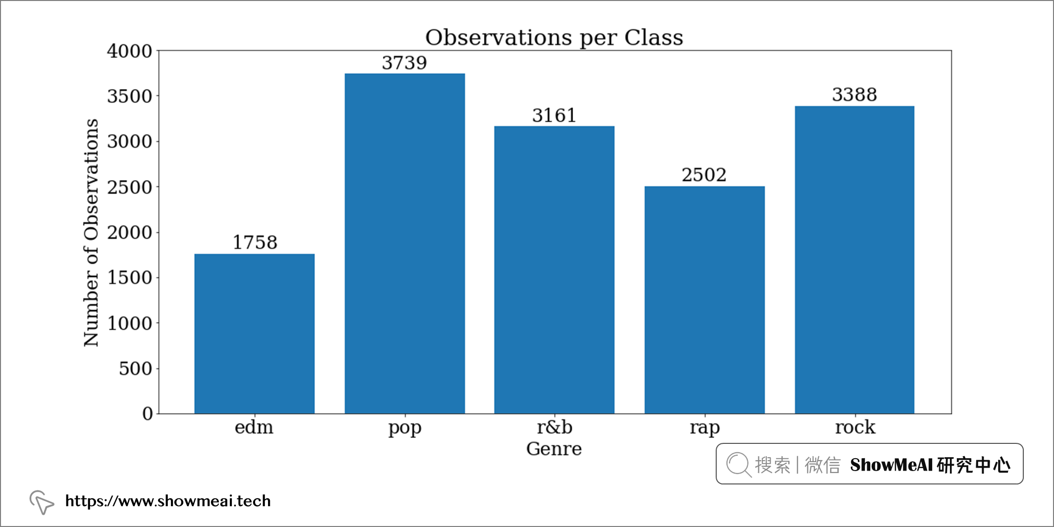
存在轻微的类别不平衡,那后续我们在交叉验证和训练测试拆分时候注意数据分层(保持比例分布) 即可。
# 把所有字段切分为音频和歌词列
audio = data[[x for x in data.columns if x.startswith("audio")]]
lyric = data[[x for x in data.columns if x.startswith("lyric")]]
# 让字段命名更简单一些
audio.columns = audio.columns.str.replace("audio_", "")
lyric.columns = lyric.columns.str.replace("lyric_", "")
💡 歌词特征&数据降维
我们的机器学习算法在处理高维数据的时候,可能会有一些性能问题,有时候我们会对数据进行降维处理。
降维的本质是将高维数据投影到低维子空间中,同时尽可能多地保留数据中的信息。关于降维大家可以查看 ShowMeAI 的算法原理讲解文章 📘 图解机器学习 | 降维算法详解
我们探索一下降维算法(PCA 和 t-SNE)在我们的歌词数据上降维是否合适,并做一点调整。
📌 PCA主成分分析
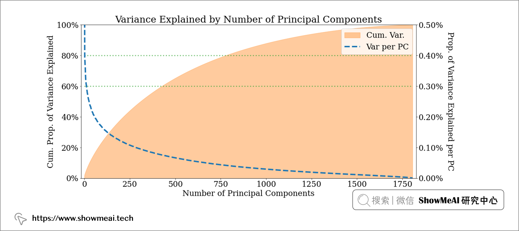
PCA是最常用的降维算法之一,我们借助这个算法可以对数据进行降维,并且看到它保留大概多少的原始信息量。例如,在我们当前场景中,如果将歌词减少到400 维,我们仍然保留了歌词中60% 的信息(方差) ;如果降维到800维,则可以覆盖 80% 的原始信息(方差)。歌词本身是很稀疏的,我们对其降维也能让模型更好地建模。
# 常规数据工具库
import pandas as pd
import numpy as np
# 绘图
import matplotlib.pyplot as plt
import matplotlib.ticker as mtick
# 数据处理
from sklearn.preprocessing import MinMaxScaler
from sklearn.decomposition import PCA

# 读取数据
data = pd.read_csv("music_data.csv")
# 切分为音频与歌词
audio = data[[x for x in data.columns if x.startswith("audio")]]
lyric = data[[x for x in data.columns if x.startswith("lyric")]]
# 特征字段
y = data.playlist_genre

# 数据幅度缩放 + PCA降维
scaler = MinMaxScaler()
audio_features = scaler.fit_transform(audio)
lyric_features = scaler.fit_transform(lyric)

pca = PCA()
lyric_pca  = pca.fit_transform(lyric_features)
var_explained_ratio = pca.explained_variance_ratio_

# Plot graph
fig, ax = plt.subplots()
# Reduce margins
plt.margins(x=0.01)
# Get cumuluative sum of variance explained
cum_var_explained = np.cumsum(var_explained_ratio)
# Plot cumulative sum
ax.fill_between(range(len(cum_var_explained)), cum_var_explained,
                alpha = 0.4, color = "tab:orange",
                label = "Cum. Var.")
ax.set_ylim(0, 1)
# Plot actual proportions
ax2 = ax.twinx()
ax2.plot(range(len(var_explained_ratio)), var_explained_ratio,
         alpha = 1, color = "tab:blue", lw  = 4, ls = "--",
         label = "Var per PC")
ax2.set_ylim(0, 0.005)

# Add lines to indicate where good values of components may be
ax.hlines(0.6, 0, var_explained_ratio.shape[0], color = "tab:green", lw = 3, alpha = 0.6, ls=":")
ax.hlines(0.8, 0, var_explained_ratio.shape[0], color = "tab:green", lw = 3, alpha = 0.6, ls=":")
# Plot both legends together
lines, labels = ax.get_legend_handles_labels()
lines2, labels2 = ax2.get_legend_handles_labels()
ax2.legend(lines + lines2, labels + labels2)
# Format axis as percentages
ax.yaxis.set_major_formatter(mtick.PercentFormatter(1))
ax2.yaxis.set_major_formatter(mtick.PercentFormatter(1))

# Add titles and labels
ax.set_ylabel("Cum. Prop. of Variance Explained")
ax2.set_ylabel("Prop. of Variance Explained per PC", rotation = 270, labelpad=30)
ax.set_title("Variance Explained by Number of Principal Components")
ax.set_xlabel("Number of Principal Components")
📌 t-SNE可视化
我们还可以更进一步,可视化数据在一系列降维过程中的可分离性。t-SNE算法是一个非常有效的非线性降维可视化方法,借助于它,我们可以把数据绘制在二维平面观察其分散程度。下面的t-SNE可视化展示了当我们使用所有1806个特征或将其减少为 1000、500、100 个主成分时,如果将歌词数据投影到二维空间中会是什么样子。
代码如下:
from sklearn.manifold import TSNE
import seaborn as sns

# Merge numeric labels with normalised audio data and lyric principal components
tsne_processed = pd.concat([
    pd.Series(y, name = "genre"),
    pd.DataFrame(audio_features, columns=audio.columns),
    # Add prefix to make selecting pcs easier later on
    pd.DataFrame(lyric_pca).add_prefix("lyrics_pc_")
          ], axis = 1)

# Get t-SNE values for a range of principal component cutoffs, 1806 is all PCs
all_tsne = pd.DataFrame()
for cutoff in ["1806", "1000", "500", "100"]:
    # Create t-SNE object
    tsne = TSNE(init = "random", learning_rate = "auto")
    # Fit on normalised features (excluding the y/label column)
    tsne_results = tsne.fit_transform(tsne_processed.loc[:, "audio_danceability":f"lyrics_pc_{cutoff}"])

    # neater graph
    if cutoff == "1806":
        cutoff = "All 1806"
    # Get results
    tsne_df = pd.DataFrame({"y":y,
                        "tsne-2d-one":tsne_results[:,0],
                       "tsne-2d-two":tsne_results[:,1],
                           "Cutoff":cutoff})
    # Store results
    all_tsne = pd.concat([all_tsne, tsne_df], axis = 0)

# Plot gridplot
g = sns.FacetGrid(all_tsne, col="Cutoff", hue = "y",
                col_wrap = 2, height = 6,
                palette=sns.color_palette("hls", 4),
               )
# Add plots
g.map(sns.scatterplot, "tsne-2d-one", "tsne-2d-two", alpha = 0.3)
# Add titles/legends
g.fig.suptitle("t-SNE Plots vs Number of Principal Components Included", y = 1)
g.add_legend()
理想情况下,我们希望看到的是,在降维到某些主成分数量(例如 cutoff = 1000)时,流派变得更加可分离。
然而,上述 t-SNE 图的结果显示,PCA 这一步不同数量的主成分并没有哪个会让数据标签更可分离。
📌 自编码器降维
实际上我们有不同的方式可以完成数据降维任务,在下面的代码中,我们提供了 PCA、截断 SVD 和 Keras 自编码器三种方式作为候选,调整配置即可进行选择。
为简洁起见,自动编码器的代码已被省略,但可以在 autoencode 内的功能 custom_functions.py 中的文件库。
# 通用库
import pandas as pd
import numpy as np
# 建模库
from sklearn.model_selection import train_test_split
from sklearn.decomposition import PCA, TruncatedSVD
from sklearn.preprocessing import LabelEncoder, MinMaxScaler
# 神经网络
from keras.layers import Dense, Input, LeakyReLU, BatchNormalization
from keras.callbacks import EarlyStopping
from keras import Model

# 定义自编码器
def autoencode(lyric_tr, n_components):
    """Build, compile and fit an autoencoder for
    lyric data using Keras. Uses a batch normalised,
    undercomplete encoder with leaky ReLU activations.
    It will take a while to train.
    --------------------------------------------------
    lyric_tr = df of lyric training data
    n_components = int, number of output dimensions
    from encoder
    """
    n_inputs = lyric_tr.shape[1]
    # 定义encoder
    visible = Input(shape=(n_inputs,))

    # encoder模块1
    e = Dense(n_inputs*2)(visible)
    e = BatchNormalization()(e)
    e = LeakyReLU()(e)
    # encoder模块2
    e = Dense(n_inputs)(e)
    e = BatchNormalization()(e)
    e = LeakyReLU()(e)
    bottleneck = Dense(n_components)(e)

    # decoder模块1
    d = Dense(n_inputs)(bottleneck)
    d = BatchNormalization()(d)
    d = LeakyReLU()(d)
    # decoder模块2
    d = Dense(n_inputs*2)(d)
    d = BatchNormalization()(d)
    d = LeakyReLU()(d)
    # 输出层
    output = Dense(n_inputs, activation='linear')(d)
    # 完整的autoencoder模型
    model = Model(inputs=visible, outputs=output)

    # 编译
    model.compile(optimizer='adam', loss='mse')
    # 回调函数
    callbacks = EarlyStopping(patience = 20, restore_best_weights = True)
    # 训练模型
    model.fit(lyric_tr, lyric_tr, epochs=200,
                        batch_size=16, verbose=1, validation_split=0.2,
             callbacks = callbacks)

    # 在降维阶段,我们只用encoder部分就可以(对数据进行压缩)
    encoder = Model(inputs=visible, outputs=bottleneck)

    return encoder

# 数据预处理函数,主要是对特征列进行降维,标签列进行编码
def pre_process(train = pd.DataFrame,
                test = pd.DataFrame,
                reduction_method = "pca",
                n_components = 400):
    # 切分X和y
    y_train = train.playlist_genre
    y_test = test.playlist_genre
    X_train = train.drop(columns = "playlist_genre")
    X_test = test.drop(columns = "playlist_genre")

    # 标签编码为数字
    label_encoder = LabelEncoder()
    label_train = label_encoder.fit_transform(y_train)
    label_test = label_encoder.transform(y_test)

    # 对数据进行幅度缩放处理
    scaler = MinMaxScaler()
    X_norm_tr = scaler.fit_transform(X_train)
    X_norm_te = scaler.transform(X_test)

    # 重建数据
    X_norm_tr = pd.DataFrame(X_norm_tr, columns = X_train.columns)
    X_norm_te = pd.DataFrame(X_norm_te, columns = X_test.columns)

    # mode和key都设定为类别型
    X_norm_tr["audio_mode"] = X_train["audio_mode"].astype("category").reset_index(drop = True)
    X_norm_tr["audio_key"] = X_train["audio_key"].astype("category").reset_index(drop = True)
    X_norm_te["audio_mode"] = X_test["audio_mode"].astype("category").reset_index(drop = True)
    X_norm_te["audio_key"] = X_test["audio_key"].astype("category").reset_index(drop = True)

    # 歌词特征
    lyric_tr = X_norm_tr.loc[:, "lyrics_aah":]
    lyric_te = X_norm_te.loc[:, "lyrics_aah":]

    # 如果使用PCA降维
    if reduction_method == "pca":
        pca = PCA(n_components)
        # 拟合训练集
        reduced_tr = pd.DataFrame(pca.fit_transform(lyric_tr)).add_prefix("lyrics_pca_")
        # 对测试集变换(降维)
        reduced_te = pd.DataFrame(pca.transform(lyric_te)).add_prefix("lyrics_pca_")

    # 如果使用SVD降维
    if reduction_method == "svd":
        svd = TruncatedSVD(n_components)
        # 拟合训练集
        reduced_tr = pd.DataFrame(svd.fit_transform(lyric_tr)).add_prefix("lyrics_svd_")
        # 对测试集变换(降维)
        reduced_te = pd.DataFrame(svd.transform(lyric_te)).add_prefix("lyrics_svd_")

    # 如果使用自编码器降维(注意,神经网络的训练时间会长一点,要耐心等待)
    if reduction_method == "keras":
        # 构建自编码器
        encoder = autoencode(lyric_tr, n_components)

        # 通过编码器部分进行数据降维
        reduced_tr = pd.DataFrame(encoder.predict(lyric_tr)).add_prefix("lyrics_keras_")
        reduced_te = pd.DataFrame(encoder.predict(lyric_te)).add_prefix("lyrics_keras_")


    # 合并降维后的歌词特征与音频特征
    X_norm_tr = pd.concat([X_norm_tr.loc[:, :"audio_duration_ms"],
                          reduced_tr
                          ], axis = 1)

    X_norm_te = pd.concat([X_norm_te.loc[:, :"audio_duration_ms"],
                           reduced_te
                           ], axis = 1)


    return X_norm_tr, label_train, X_norm_te, label_test, label_encoder


# 分层切分数据
train_raw, test_raw = train_test_split(data, test_size = 0.2,
                                       shuffle = True, random_state = 42, # random, reproducible split
                                       stratify = data.playlist_genre)
# 设定降维最终维度
n_components = 500
# 选择降维方法,候选: "pca", "svd", "keras"
reduction_method = "pca"

# 完整的数据预处理
X_train, y_train, X_test, y_test, label_encoder = pre_process(train_raw, test_raw,
                                                      reduction_method = reduction_method,
                                                     n_components = n_components)
上述过程之后我们已经完成对数据的标准化、编码转换和降维,接下来我们使用它进行建模。
💡 建模和超参数优化
📌 构建模型
在实际建模之前,我们要先选定一个评估指标来评估我们模型的性能,也方便指导进一步的优化。由于我们数据最终的标签『流派/类别』略有不平衡,宏观 F1 分数(macro f1-score) 可能是一个不错的选择,因为它平等地评估了类别的贡献。我们在下面对这个评估准则进行定义,也敲定 LightGBM 模型的部分超参数。
from sklearn.metrics import f1_score

# 定义评估准则(Macro F1)
def lgb_f1_score(preds, data):
    labels = data.get_label()
    preds = preds.reshape(5, -1).T
    preds = preds.argmax(axis = 1)
    f_score = f1_score(labels , preds,  average = 'macro')
    return 'f1_score', f_score, True

# 用于编译的参数
fixed_params = {
        'objective': 'multiclass',
        'metric': "None",   # 我们自定义的f1-score可以应用
        'num_class': 5,
        'verbosity': -1,
}
LightGBM 带有大量可调超参数,这些超参数对于最终效果影响很大。
关于 LightGBM 的超参数细节详细讲解,欢迎大家查阅 ShowMeAI 的文章:
下面我们会基于Optuna这个工具库对 LightGBM 的超参数进行调优,我们需要在 param 定义超参数的搜索空间,在此基础上 Optuna 会进行优化和超参数的选择。
# 建模
from sklearn.model_selection import StratifiedKFold
import lightgbm as lgb
from optuna.integration import LightGBMPruningCallback

# 定义目标函数
def objective(trial, X, y):
    # 候选超参数
    param = {**fixed_params,
        'boosting_type': 'gbdt',
        'num_leaves': trial.suggest_int('num_leaves', 2, 3000, step = 20),
        'feature_fraction': trial.suggest_float('feature_fraction', 0.2, 0.99, step = 0.05),
        'bagging_fraction': trial.suggest_float('bagging_fraction', 0.2, 0.99, step = 0.05),
        'bagging_freq': trial.suggest_int('bagging_freq', 1, 7),
        'min_child_samples': trial.suggest_int('min_child_samples', 5, 100),
        "n_estimators": trial.suggest_int("n_estimators", 200, 5000),
        "learning_rate": trial.suggest_float("learning_rate", 0.01, 0.3),
        "max_depth": trial.suggest_int("max_depth", 3, 12),
        "min_data_in_leaf": trial.suggest_int("min_data_in_leaf", 5, 2000, step=5),
        "lambda_l1": trial.suggest_float("lambda_l1", 1e-8, 10.0, log=True),
        "lambda_l2": trial.suggest_float("lambda_l2", 1e-8, 10.0, log=True),
        "min_gain_to_split": trial.suggest_float("min_gain_to_split", 0, 10),
        "max_bin": trial.suggest_int("max_bin", 200, 300),
    }

    # 构建分层交叉验证
    cv = StratifiedKFold(n_splits = 5, shuffle = True)
    # 5组得分
    cv_scores = np.empty(5)

    # 切分为K个数据组,轮番作为训练集和验证集进行实验
    for idx, (train_idx, test_idx) in enumerate(cv.split(X, y)):
        # 数据切分
        X_train_cv, X_test_cv = X.iloc[train_idx], X.iloc[test_idx]
        y_train_cv, y_test_cv = y[train_idx], y[test_idx]

        # 转为lightgbm的Dataset格式
        train_data = lgb.Dataset(X_train_cv, label = y_train_cv, categorical_feature="auto")
        val_data = lgb.Dataset(X_test_cv, label = y_test_cv,  categorical_feature="auto",
                              reference = train_data)

        # 回调函数
        callbacks = [
            LightGBMPruningCallback(trial, metric = "f1_score"),
                     # 间歇输出信息
                    lgb.log_evaluation(period = 100),
                     # 早停止,防止过拟合
                    lgb.early_stopping(50)]

        # 训练模型
        model = lgb.train(params = param,  train_set = train_data,
                          valid_sets = val_data,
                          callbacks = callbacks,
                          feval = lgb_f1_score # 自定义评估准则
                         )

        # 预估
        preds = np.argmax(model.predict(X_test_cv), axis = 1)
        # 计算f1-score
        cv_scores[idx] = f1_score(y_test_cv, preds, average = "macro")

    return np.mean(cv_scores)
📌 超参数优化
我们在上面定义完了目标函数,现在可以使用 Optuna 来调优模型的超参数了。
# 超参数优化
import optuna

# 定义Optuna的实验次数
n_trials = 200
# 构建Optuna study去进行超参数检索与调优
study = optuna.create_study(direction = "maximize", # 最大化交叉验证的F1得分
                            study_name = "LGBM Classifier",
                           pruner=optuna.pruners.HyperbandPruner())
func = lambda trial: objective(trial, X_train, y_train)
study.optimize(func, n_trials = n_trials)
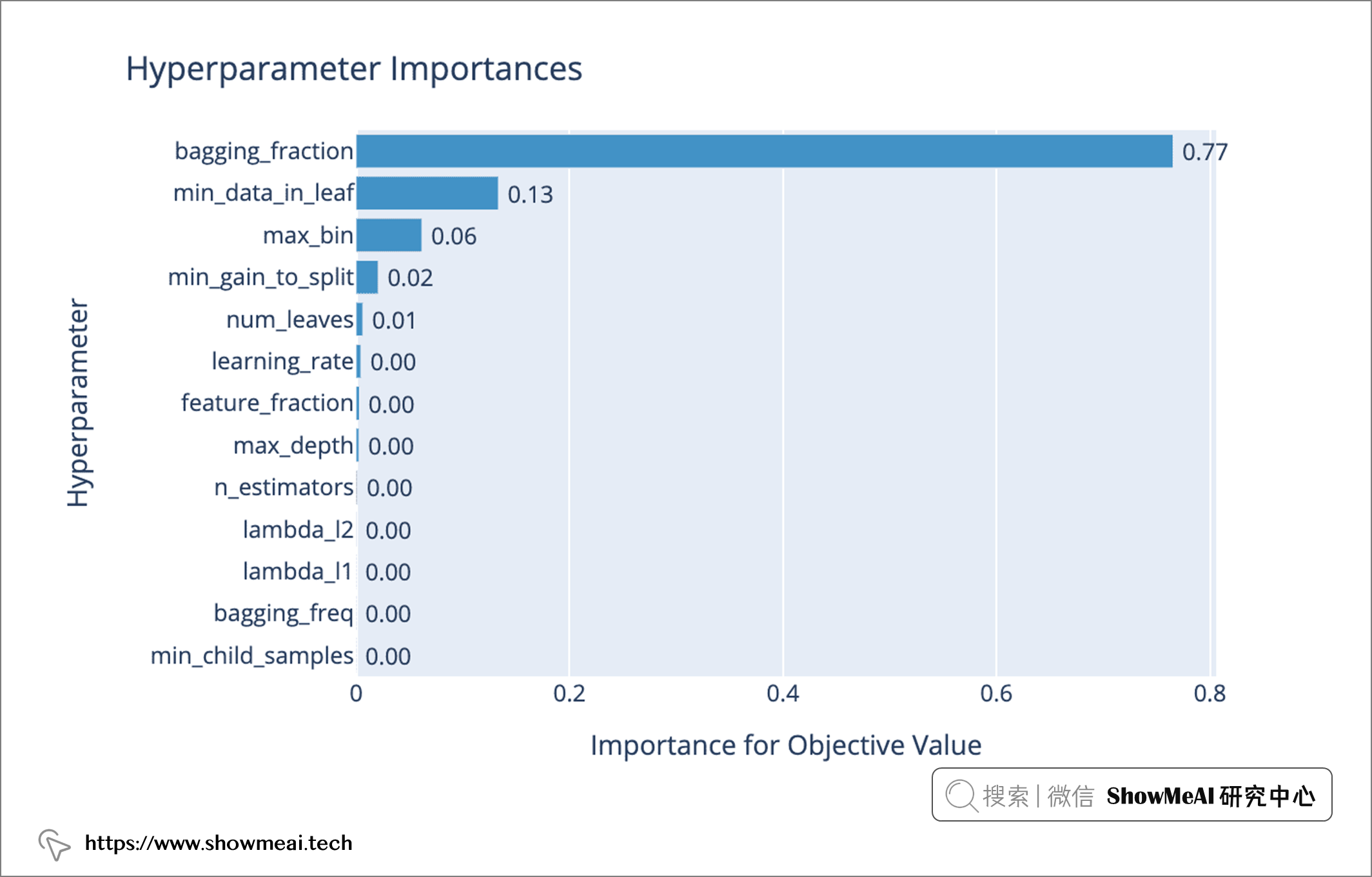
然后,我们可以使用 📘 Optuna 的可视化模块 对不同超参数组合的性能进行可视化查看。例如,我们可以使用 plot_param_importances(study) 查看哪些超参数对模型性能/影响优化最重要。
plot_param_importances(study)
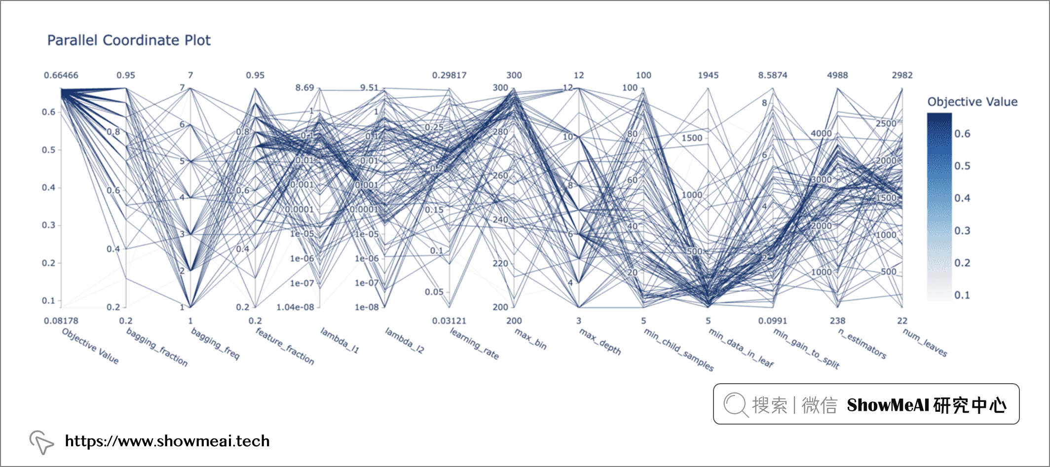
我们也可以使用 plot_parallel_coordinate(study)查看尝试了哪些超参数组合/范围可以带来高评估结果值(好的效果性能)。
plot_parallel_coordinate(study)
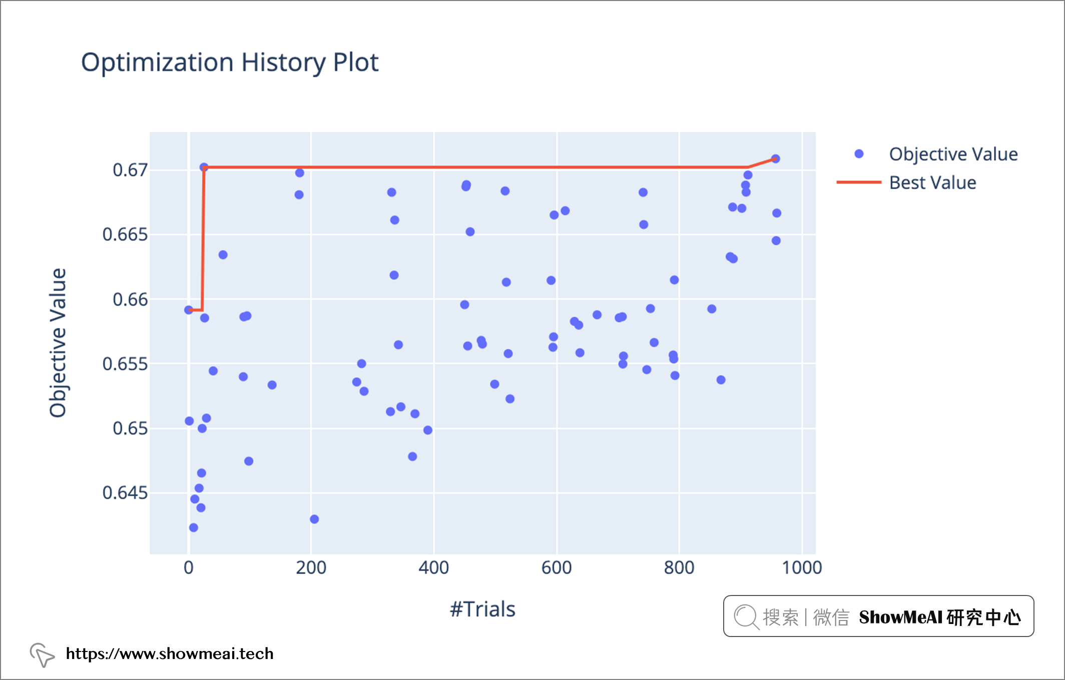
然后我们可以使用 plot_optimization_history 查看历史情况。
plot_optimization_history(study)
在Optuna完成调优之后:
- 最好的超参数存储在
study.best_params属性中。我们把模型的最终参数params定义为params = {**fixed_params, **study.best_params}即可,如后续的代码所示。 - 当然,你也可以缩小搜索空间/超参数范围,进一步做精确的超参数优化。
# 最佳模型实验
cv = StratifiedKFold(n_splits = 5, shuffle = True)
# 5组得分
cv_scores = np.empty(5)

# 切分为K个数据组,轮番作为训练集和验证集进行实验
for idx, (train_idx, test_idx) in enumerate(cv.split(X, y)):
    # 数据切分
    X_train_cv, X_test_cv = X.iloc[train_idx], X.iloc[test_idx]
    y_train_cv, y_test_cv = y[train_idx], y[test_idx]

    # 转为lightgbm的Dataset格式
    train_data = lgb.Dataset(X_train_cv, label = y_train_cv, categorical_feature="auto")
    val_data = lgb.Dataset(X_test_cv, label = y_test_cv,  categorical_feature="auto",
                          reference = train_data)

    # 回调函数
    callbacks = [
        LightGBMPruningCallback(trial, metric = "f1_score"),
                 # 间歇输出信息
                lgb.log_evaluation(period = 100),
                 # 早停止,防止过拟合
                lgb.early_stopping(50)]

    # 训练模型
    model = lgb.train(params = {**fixed_params, **study.best_params},  train_set = train_data,
                      valid_sets = val_data,
                      callbacks = callbacks,
                      feval = lgb_f1_score # 自定义评估准则
                     )

    # 预估
    preds = np.argmax(model.predict(X_test_cv), axis = 1)
    # 计算f1-score
    cv_scores[idx] = f1_score(y_test_cv, preds, average = "macro")
💡 最终评估
通过上述过程我们就获得了最终模型,让我们来评估一下吧!
# 预估与评估训练集
train_preds = model.predict(X_train)
train_predictions = np.argmax(train_preds, axis = 1)
train_error = f1_score(y_train, train_predictions, average = "macro")

# 交叉验证结果
cv_error = np.mean(cv_scores)

# 评估测试集
test_preds = model.predict(X_test)
test_predictions = np.argmax(test_preds, axis = 1)
test_error = f1_score(y_test, test_predictions, average = "macro")

# 存储评估结果
results = pd.DataFrame({"n_components": n_components,
                        "reduction_method": reduction_method,
                        "train_error": train_error,
                        "cv_error": cv_error,
                        "test_error": test_error,
                        "n_trials": n_trials
                       }, index = [0])
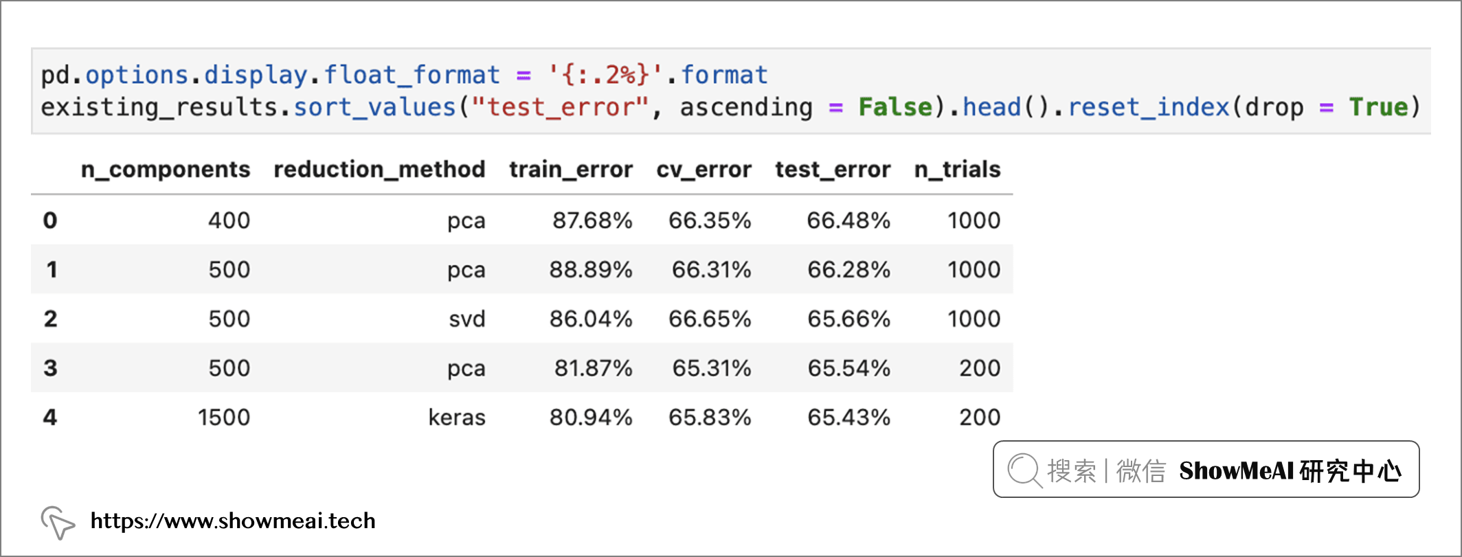
我们可以实验和比较不同的降维方法、降维维度,再调参查看模型效果。如下图所示,在我们当前的尝试中,PCA降维到 400 维产出最好的模型 ——macro f1-score 为66.48%。
在本篇内容中, ShowMeAI 展示了基于歌曲信息与文本对其进行『流派』分类的过程,包含对文本数据的处理、特征工程、模型建模和超参数优化等。大家可以把整个pipeline作为一个模板来应用在其他任务当中。
- 📘 图解数据分析:从入门到精通系列教程: https://www.showmeai.tech/tutorials/3
- 📘 数据科学工具库速查表 | Pandas 速查表: https://www.showmeai.tech/article-detail/101
- 📘 图解机器学习算法 | 降维算法详解: https://www.showmeai.tech/article-detail/198
- 📘 图解机器学习算法 | LightGBM模型详解: https://www.showmeai.tech/article-detail/195
- 📘 机器学习实战 | LightGBM建模应用详解: https://www.showmeai.tech/article-detail/205
- 📘 Optuna 的可视化模块
- 📘 Akiba,T., Sano, S., Yanase, T., Ohta, T., & Koyama, M. (2019, July). Optuna: A next-generation hyperparameter optimization framework. In Proceedings of the 25th ACM SIGKDD international conference on knowledge discovery & data mining (pp. 2623–2631).
- 📘 Autoencoder Feature Extractions
- 📘 Kaggler’s Guide to LightGBM Hyperparameter Tuning with Optuna in 2021
- 📘 You Are Missing Out on LightGBM. It Crushes XGBoost in Every Aspect

- 赞
- 收藏
- 评论
- 分享
- 举报
Recommend
-
8
本文适合有 C++ 基础的朋友 本文作者:HelloGitHub- Anthony HelloGitHub 推出的《讲解开源项目》系列,本...
-
3
超惊艳3D!平行世界什么样?这100位艺术大佬用作品直接回答 3D / 动画 /
-
4
倒计时 1 天!赛博北京,一场元宇宙世界的艺术聚会链得得 ChainDD.com |得区块链者得天下|摘要:2021 年 8 月 7 日,由链得得、钛媒体、CryptoC、风潮、元気星空、C&L; 空间联合发起的第一届“赛博北京·数字艺术节”将在北京大兴开幕,数字...
-
1
当3D技术迈进建筑与艺术的浪漫世界 3D视觉艺术 / 建筑设计...
-
6
这个品牌大胆起来,比庞宽更“艺术” 作者: River ...
-
2
这个好看的文字排版方法,小白也能学会! 7月 22, 2022 发表于: 视觉设计.
-
5
AI 音辨世界:艺术小白的我,靠这个AI模型,速识音乐流派选择音乐 ...
-
3
世界互联网大会上,唯一艺术重磅发布数藏云“唯艺云”-品玩 业界动态 世界互联网大会上,唯一艺术重磅发布数藏云“唯艺云”
-
4
每到11月,作为一个电商行业的小白优化师,我就开始瑟瑟发抖。为了冲刺双11...
-
9
C站:Civitai,一个AI绘画艺术模型下载与分享社区 5月 22, 2023 发表于: 视觉设计.
About Joyk
Aggregate valuable and interesting links.
Joyk means Joy of geeK