Stable Fluids with three.js

7/31/2022

I decided to study fluid simulation because I need it for my job.
I will discretize and implement the Navier-Stokes equations.
I heard that the method called Stable Fluids is commonly used for real-time rendering, so I did a lot of research based on that.
I only have a limited knowledge of high school mathematics, so I found many unfamiliar terms and characters in the equation, and it was more difficult to understand than I had imagined, but I think I managed to at least understand it, so I would like to explain it in my own way.

How to implement

The implementation will be done in three.js, a WebGL library.
The important thing is the combination of fbo and the calculation in the shader, so there is little need to use the library.
(The advantage is that it is easy to implement for use in a project.)
I'm using three.js because personal preference, so I think it can be replaced by raw WebGL or something else.
demo

Introduction

What is Navie-Stokes equation?

"In physics, the Navier–Stokes equations are certain partial differential equations which describe the motion of viscous fluid substances, named after French engineer and physicist Claude-Louis Navier and Anglo-Irish physicist and mathematician George Gabriel Stokes." (wikipedia)

It is an equation of fluid dynamics presented by mathematicians Navier and Stokes.
It looks very difficult and I had no idea what ∇ in particular was about.
But don't worry. It can be discretized and in concrete implementation it is a combination of four arithmetic operations.

Before we get into the equation, let me first introduce the variables that appear in the equation.

Variables

u⃗ \vec{\boldsymbol{u}}u
It is the velocity vector of the fluid, denoted u⃗=(ux,uy) \vec{\boldsymbol{u}} = (\boldsymbol{u_x}, \boldsymbol{u_y})u=(ux​,uy​) for 2D, u⃗=(ux,uy,uz) \vec{\boldsymbol{u}} = (\boldsymbol{u_x}, \boldsymbol{u_y}, \boldsymbol{u_z})u=(ux​,uy​,uz​) for 3D.
This Navie-Stokes equation is used to solve for the final velocity u⃗ \vec{\boldsymbol{u}}u.

ppp
It is a scalar variable that represents pressure. (Scalar variables are float variables in glsl).
pppis another unknown variable that we'll need to solve from now on.

ν\nuν
This is a constant that represents viscosity.
Since it is a constant, you can put in any value you like when calculating this term.
The larger the value, the more viscous it is.

F⃗\vec{F}F
A vector representing the external force. You must provide this value yourself. In this case, we will implement the mouse movement as an external pressure.

ttt
Elapsed time.


Now, we have one equation but two unknown variables.
This makes it impossible to solve, so we solve for ppp by solving the equation for incompressibility in a series, and then solve for u⃗ \vec{\boldsymbol{u}}u based on that.

This is the equation for incompressibility and is called the equation of continuity.
Intuitively, it means that volume and mass remain the same whether the flow is flowing or stationary.

Meaning of each term

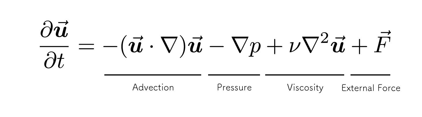
External force term
Add force applied from the outside (in implementation, calculated by mouse difference)

Advection term
Follow the fluid flow.

Viscosity term
This section shows the viscosity of the fluid.
I think it is OK to skip this part of the fluid implementation for visualization purposes.
(It is as heavy a process as the pressure term.)

Pressure term
Calculates the forces of fluids pushing against each other
(under conditions of non-compression).

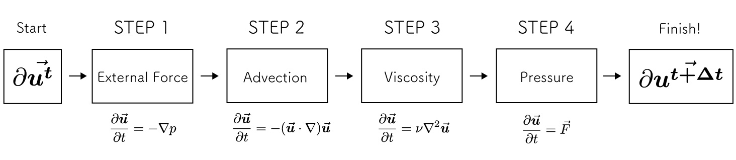
We will solve for these terms and finally calculate the velocity of the next step.
We will use a method called Stable Fluids that solves each term one at a time.

Assumptions

To solve this equation, here are a few assumptions.

Finite Difference Method

The Navier-Stokes equation is a partial differential equation, but of course the frame rate and the amount of pixels are limited, so the finite difference method is used to solve it.
In this case, we will solve the equation with Δx=Δy=1 \Delta x = \Delta y = 1Δx=Δy=1 and Δt=1/60 \Delta t = 1/60Δt=1/60.

Euler method

There are two methods for observing fluid flow: the Eulerian method and the Lagrangian method.
The Eulerian method observes the fluid as each cell enters its own cell, and the The Lagrangian method looks at the position where one's flow goes from the fluid grain perspective.
In this implementation, the Eulerian method is a better fit since the calculation is done in the fragment shader.
We will implement this by viewing each pixel as a cell where the fluid goes and comes.

Vector calculus

Vector and scalar fields

Vector and scalar variables are laid out everywhere in space. A good example of vector and scalar fields that we are familiar with in everyday life is a weather map. You can imagine a map with temperature (scalar), atmospheric pressure (scalar), and wind direction (vector) all laid out on the map.

Nabla

This calculation uses not only the time derivative(∂/∂t\partial / \partial t∂/∂t) but also the spatial derivative many times.
The spatial derivative is, in finite-difference terms, the difference between neighboring cells.
The value of your cell is not used, but that of both neighbors.
The central difference, which takes the difference between two neighboring values without using the value of one's own cell, seems to be more precise.
We will solve it for all but the advection term in this way.

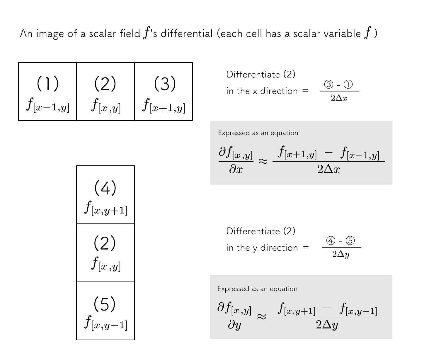
The symbol nabla∇\nabla∇, which appears many times in the Navier-Stokes equations, refers to the operator of spatial differentiation.

∇\nabla∇ is just a symbol for concisely expressing the differential notation of vector and scalar fields, so there is no need to be defensive about it being a difficult symbol.
It is a notation used when you want to see the difference between the top, bottom, left, right (or even the depth).

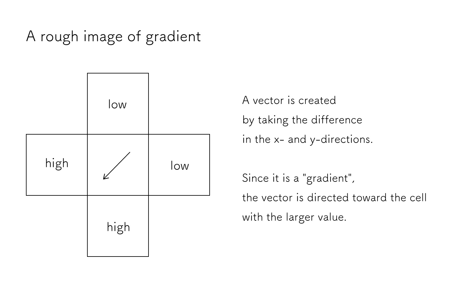
Gradient

A closer look at the ∇p\nabla p∇p:

The approximation is

A new vector is created by taking the amount of change in ppp in the left, right, top and bottom cells.
This vector is called the gradient because it represents the slope at that point.

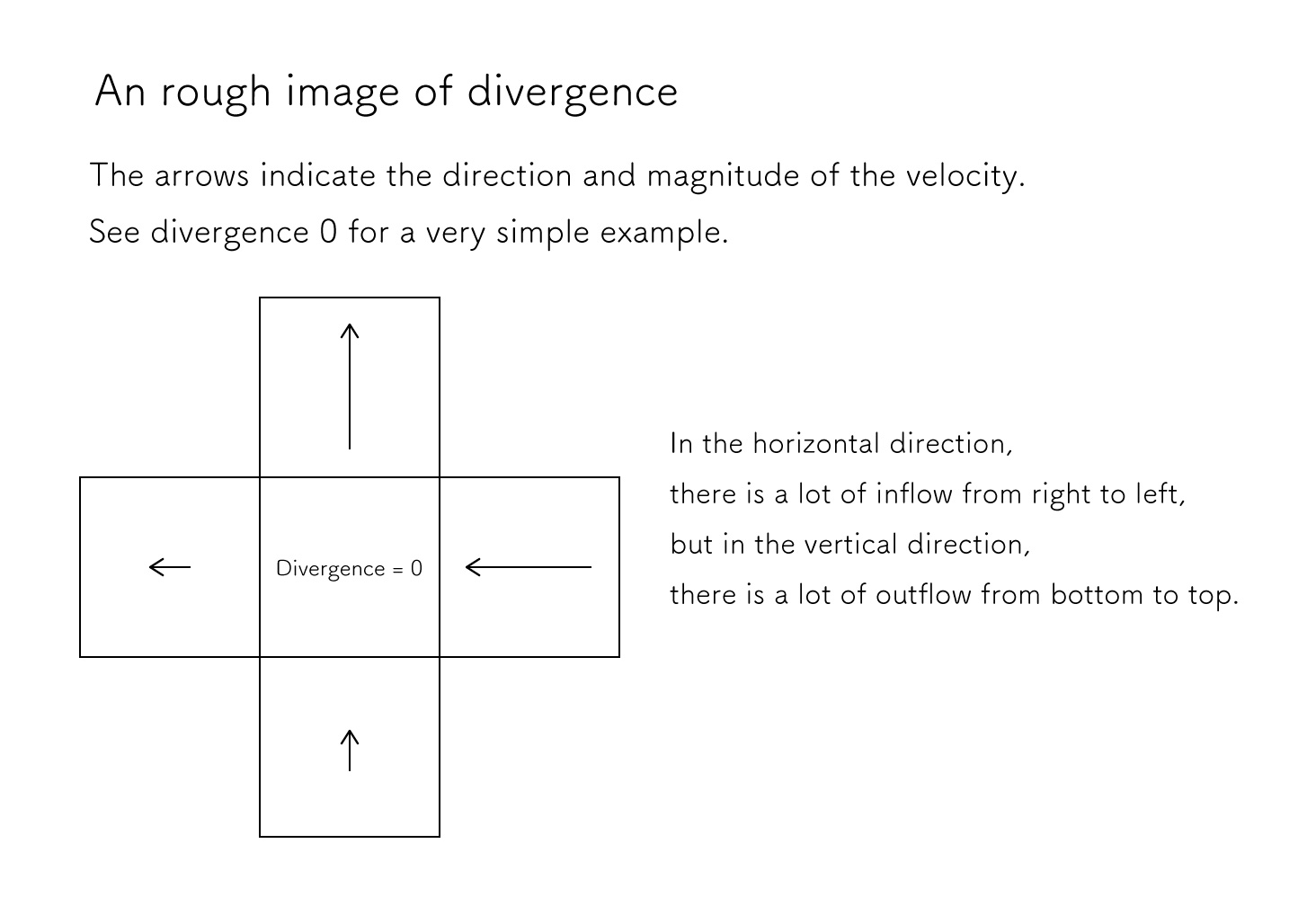
Divergence

Divergence is how much fluid flows in and out.
Divergence >0> 0>0 means more outflow and divergence <0< 0<0 means more inflow.
In other words, the continuity equation ∇⋅u⃗=0 \nabla \cdot \vec{u} = 0∇⋅u=0 means that the inflow and outflow are equal to zero.
If we focus on a small cell with a tank full of fluid, we can imagine that the amount of fluid entering and leaving the cell is the same.

Since this is in inner product notation, the calculation is performed in the same way as the inner product of a two-dimensional vector.
The result is also a scalar, just like the inner product.

The approximation is

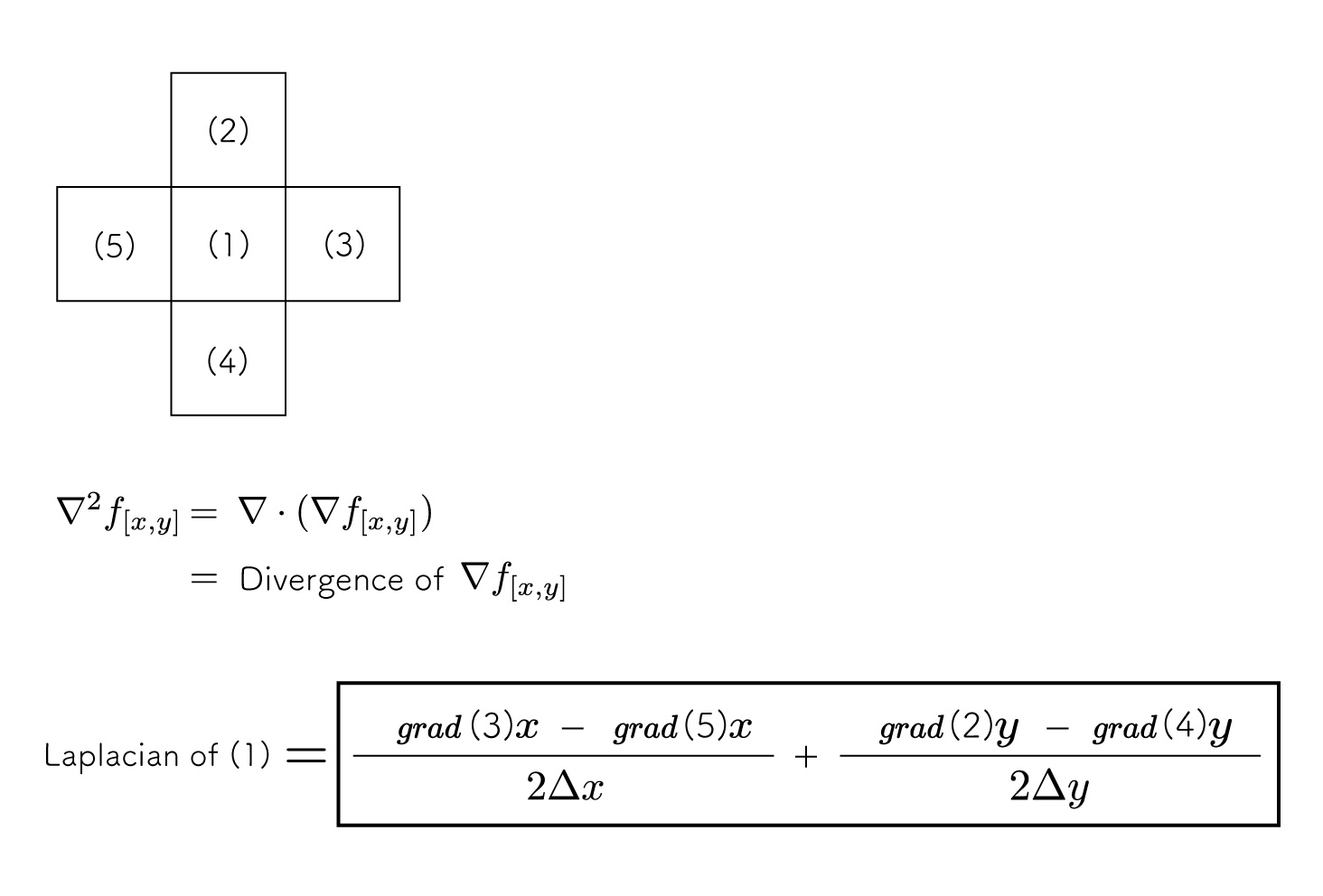
Laplacian

The Laplacian is the gradient with respect to a scalar field plus a further divergence.
The differential operator of the Laplacian is denoted by ∇2 \nabla^2∇2.

The divergence is

So the Laplacian fff of the coordinates (x, y) is

The approximation of the gradient fff is

So the Laplacian fff of the coordinates (x, y) is

If Δx=Δy\Delta x = \Delta yΔx=Δy

The above equation is too detailed to read, so we will use a simple figure.

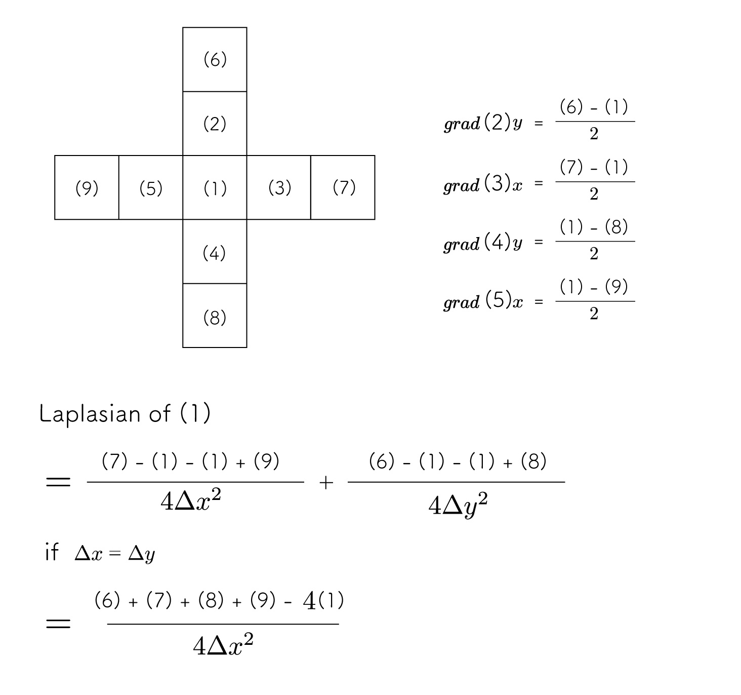
I think I was able to visualize the Laplacian.
This discrete expression of the Laplacian is used to calculate the viscosity term and pressure ppp.

The above is the prior knowledge for actual calculation.
Next, we will finally move on to the implementation!

Implementation

Preparation

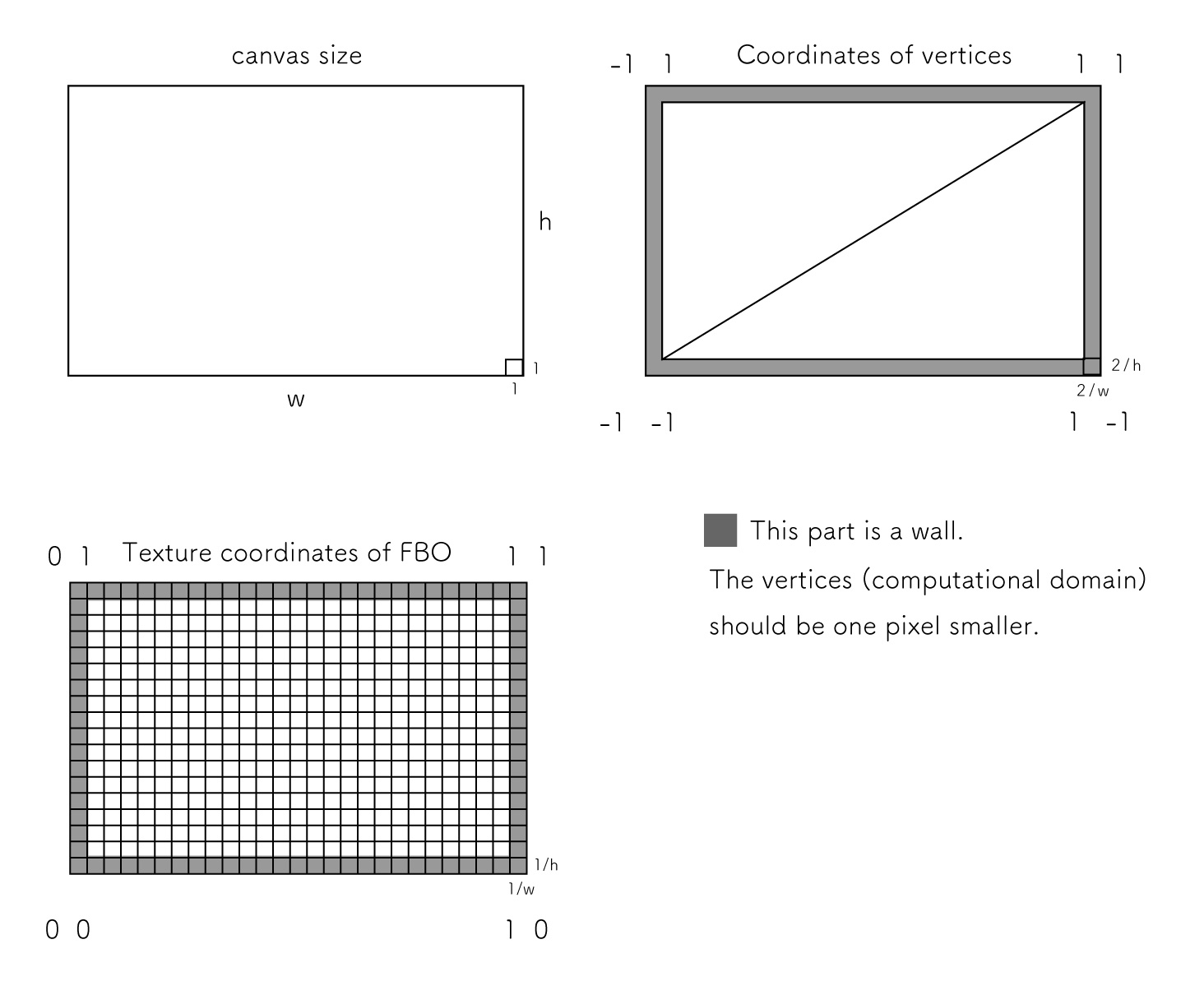
First, let's check the size of the canvas, the placement of the plane vertices, and the size of the fbo.
It will be less confusing if you draw a diagram like the one above before starting the implementation.
We will write the code based on this diagram.

The edge of the canvas should be the wall of the fluid.
This is called a boundary condition, and setting it will stabilize the fluid.
This is the gray area a diagram, but this time we will not calculate this area, but assume it is where the convergence to zero occurs

// Resolution
// Smaller as it will be very heavy depending on specs
const resolution = 0.25;
const width = Math.round(canvas.width * resolution);
const height = Math.round(canvas.height * resolution);

// (length of 1 cell) / (overall length)
const cellScale = new THREE.Vector2(1 / width, 1 / height);

// vertex
// size excluding edges
const planeG = new THREE.PlaneBufferGeometry(
 2 - cellScale.x * 2,
 2 - cellScale.y * 2
)

// number of pixels in fbo
const fboSize = new THREE.Vector2(
  width,
  height
);

const fbos = {
  // The velocity. Use alternating for clarity.
  vel_0: null
  vel_1: null,

  // Calculate the viscosity term. Use alternating.
  vel_viscous0: null,
  vel_viscous1: null
  // The divergence values for pressure calculation
  div: null,

  // Calculate the Pressure. Use alternately.
  pressure_0: null,
  pressure_1: null
}

for(let key in fbos){
  fbos[key] = new THREE.WebGLRenderTarget({
    fboSize.x,
    fboSize.y,
    {
      type: THREE.FloatType
    }
  })
}

External force

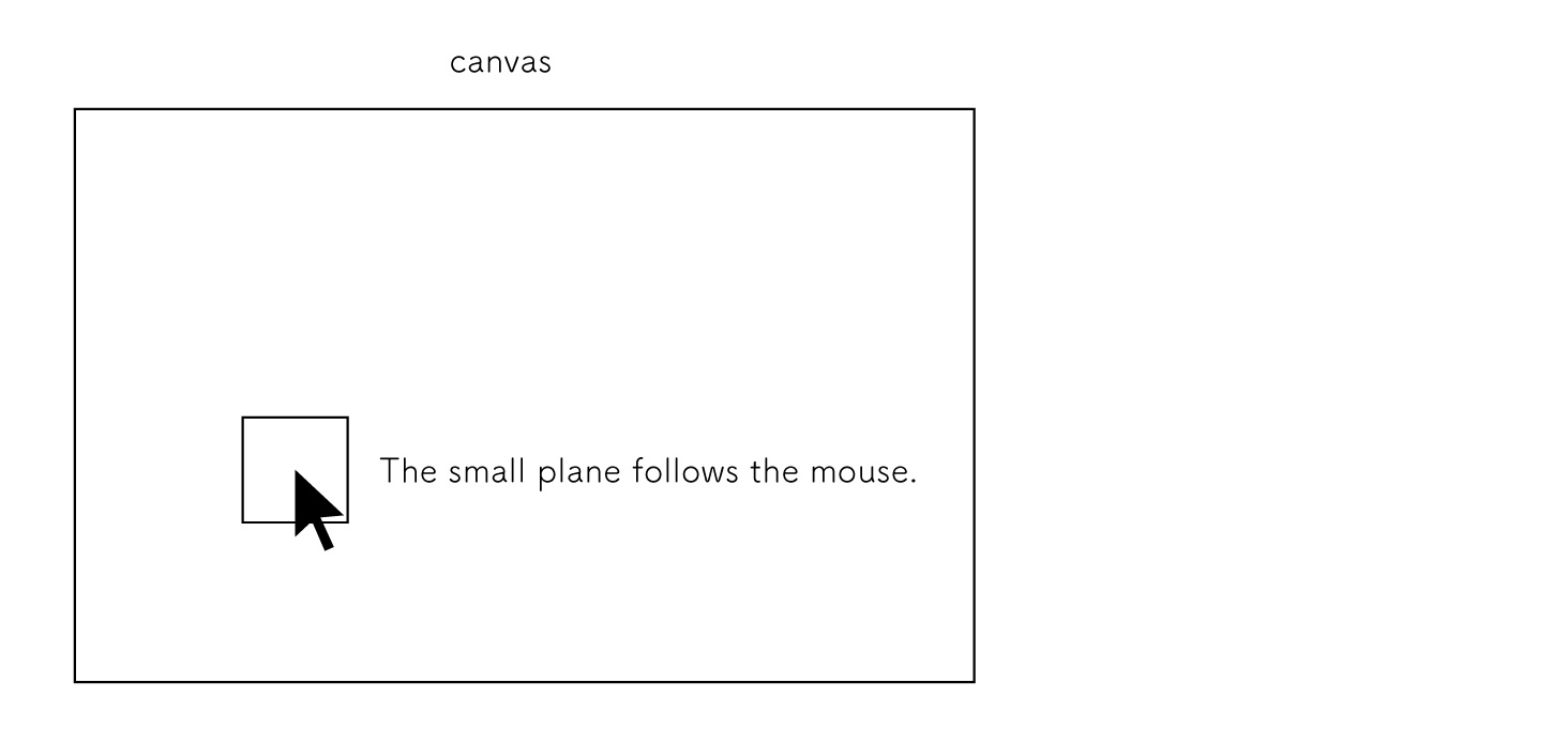
External pressure is simply implemented by taking the mouse position and the amount of movement and adding it to the velocity.
The following code is a simple example of processing the fragment shader of a mouse plane.

uniforms sampler2D velocity;
uniforms vec2 force;
uniforms vec2 fboSize;
varying vec2 vUv;

void main(){
  vec2 st = gl_FragCoord.xy / fboSize;
  vec2 oldVel = sampler2D(velocity, st);

  // The more mouse-centered, the larger the value.
  float intensity = 1.0 - min(length(vUv * 2.0 - 1.0), 1.0);
  // Just add the size of the mouse at the uv point to the velocity.
  gl_FragColor = vec4(oldVel + intensity * force, 0, d);
}

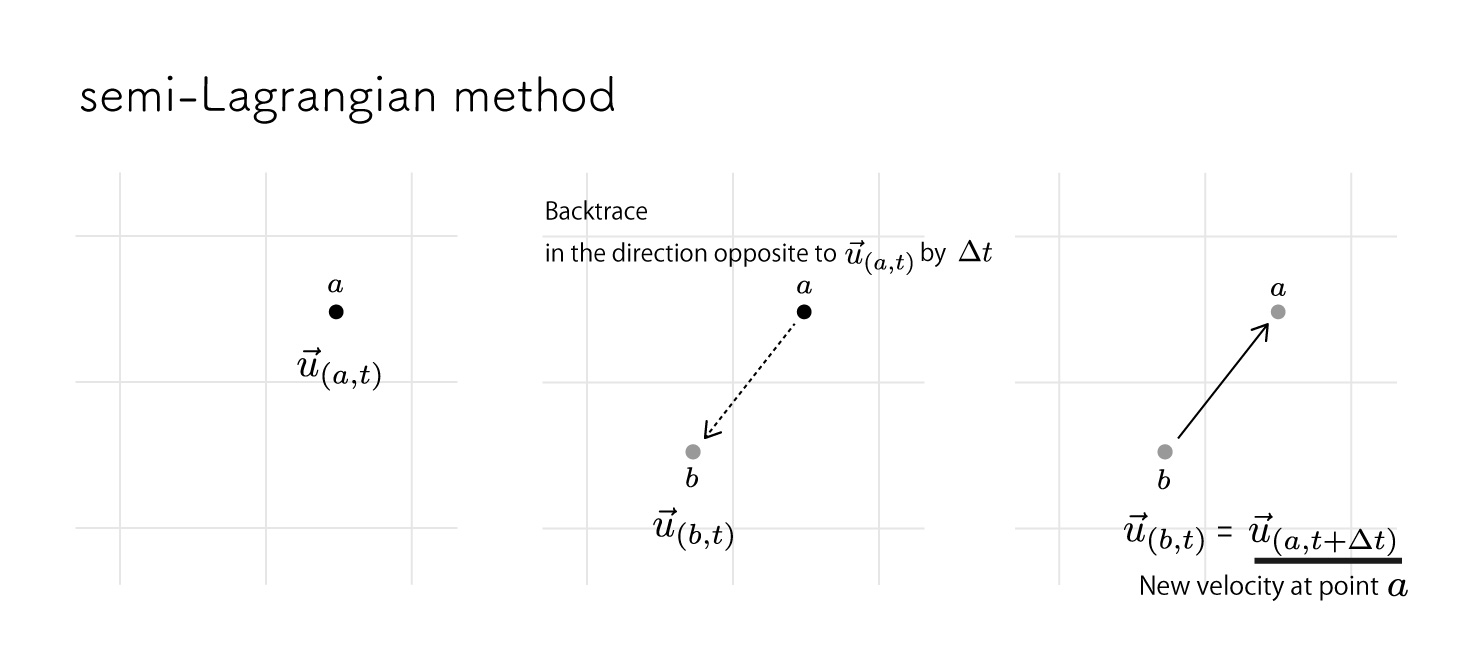
Advection

Next, we will calculate advection.

As it turns out, it is easier and more stable to use the semi-Lagrangian method, which is a compromise between the Lagrangian and Eulerian methods.
There are various ways to do this with the Euler method, but they have limited conditions and are difficult to stabilize.

The semi-Lagrangian method is a method in which the velocity u(b,t)u_{(b, t)} u(b,t)​ at point bbb is taken as the velocity u(a,t+Δt)u_{(a, t+\Delta t)} u(a,t+Δt)​ of the next step at calculation point aaa, after backtracing in the direction of u(a,t)u_{(a, t)} u(a,t)​ by Δt\Delta tΔt from calculation point aaa.

uniform sampler2D velocity;
uniform float dt;
uniform vec2 fboSize;
varying vec2 uv;

void main(){
  vec2 ratio = max(fboSize.x, fboSize.y) / fboSize;
  vec2 vel = texture2D(velocity, uv).xy;
  vec2 uv2 = uv - vel * dt * ratio;
  vec2 newVel = texture2D(velocity, uv2).xy;
  gl_FragColor = vec4(newVel, 0.0, 0.0);
}

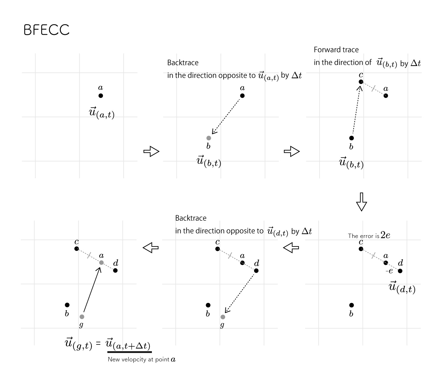
However, this method assumes that the advection is linear. If the backtrace should be curvilinear, this would result in errors.
BFECC (Back and Forth Error Compensation and Correction) is a method that attempts to correct for this error as much as possible.

void main(){
  vec2 ratio = max(fboSize.x, fboSize.y) / fboSize;

  vec2 spot_new = uv;
  vec2 vel_old = texture2D(velocity, uv).xy;
  // back trace
  vec2 spot_old = spot_new - vel_old * dt * ratio;
  vec2 vel_new1 = texture2D(velocity, spot_old).xy;

  // forward trace
  vec2 spot_new2 = spot_old + vel_new1 * dt * ratio;
        
  vec2 error = spot_new2 - spot_new;

  vec2 spot_new3 = spot_new - error / 2.0;
  vec2 vel_2 = texture2D(velocity, spot_new3).xy;

  // back trace 2
  vec2 spot_old2 = spot_new3 - vel_2 * dt * ratio;

  vec2 newVel2 = texture2D(velocity, spot_old2).xy; 
  gl_FragColor = vec4(newVel2, 0.0, 0.0);

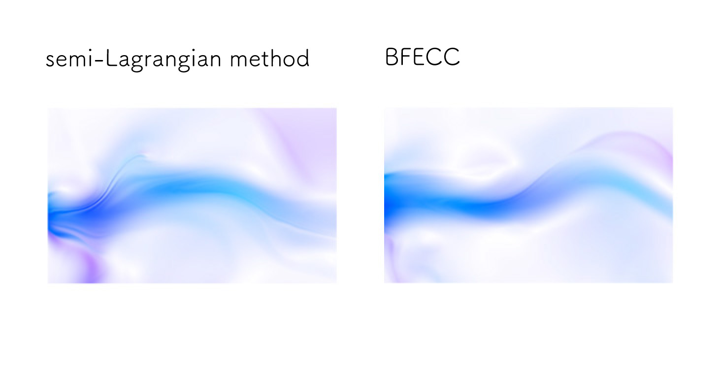
You can see the difference on the demo by toggling in a top right controls.

Viscousity

The viscosity term is a little more difficult.
We will look at it in a little bit as we solve the equation.

Taking the approximation of TTT and u⃗\vec{u}u

Taking the approximation under Δx=Δy=1\Delta x = \Delta y= 1 Δx=Δy=1
(Use the LaplacianLaplacian approximation)

What we need to find here is u⃗(x,y,t+Δt)\vec{u}_{(x, y, t + \Delta t)}u(x,y,t+Δt)​, but because of the Laplacian ∇2 \nabla^2∇2, we also need u⃗\vec{u}u of the surrounding cells at t+Δtt + \Delta tt+Δt.
When we need other future values to find a future value, we use an iterative method to converge to the correct value as much as possible. In this case, we will use the Jacobi method because it is the only way to iterate using two fbo's to perform the calculation in the fragment shader.
The Jacobi method is suitable for parallel processing.
(For cpu calculations such as javascript, the Gauss-Seidel method, which requires only one array of values, is more suitable.)

precision highp float;
uniform sampler2D velocity;
uniform sampler2D velocity_new;
uniform float v;
uniform vec2 px;
uniform float dt;

varying vec2 uv;

void main(){
    vec2 old = texture2D(velocity, uv).xy;
    vec2 new0 = texture2D(velocity_new, uv + vec2(px.x * 2.0, 0)).xy;
    vec2 new1 = texture2D(velocity_new, uv - vec2(px.x * 2.0, 0)).xy;
    vec2 new2 = texture2D(velocity_new, uv + vec2(0, px.y * 2.0)).xy;
    vec2 new3 = texture2D(velocity_new, uv - vec2(0, px.y * 2.0)).xy;

    vec2 new = 4.0 * old + v * dt * (new0 + new1 + new2 + new3);
    new /= 4.0 * (1.0 + v * dt);
    
    gl_FragColor = vec4(new, 0.0, 0.0);
}

// In order to perform iterative calculations, the fbo that stores the calculation results and the fbo of the latest calculation results are alternately replaced.
let fbo_in, fbo_out;
this.uniforms.v.value = viscous;
for(var i = 0; i < iterations; i++){
    if(i % 2 == 0){
        fbo_in = this.props.output0;
        fbo_out = this.props.output1;
    } else {
        fbo_in = this.props.output1;
        fbo_out = this.props.output0;
    }

    this.uniforms.velocity_new.value = fbo_in.texture;
    this.props.output = fbo_out;
    this.uniforms.dt.value = dt;
}

Pressure

The pressure term is also a bit difficult to solve. (but it is the last calculation finally !)
Since there are two variables in the pressure term, ppp and u⃗\vec{u}u at t+Δtt + \Delta tt+Δt, we will use the continuous equation ∇⋅u⃗=0\nabla \cdot \vec{u} = 0∇⋅u=0 to solve it.
We will first find ppp and then u⃗\vec{u}u.

Taking an approximation:

Calculate divergence on both sides.

Since the assumption is that ∇⋅u⃗(x,y,t+Δt)=0\nabla \cdot \vec{u}_{(x, y, t + \Delta t)} = 0∇⋅u(x,y,t+Δt)​=0 due to the non-compression condition

Now that we have the Laplacian ∇2\nabla^2∇2, we will use the iterative method to approximate ppp as well as the viscosity term.

Taking the approximation under Δx=Δy=1\Delta x = \Delta y= 1 Δx=Δy=1

After solving for this value of ppp using the iterative method, we can calculate the new velocity u⃗(x,y,t+Δt)\vec{u}_{(x, y, t+\Delta t)}u(x,y,t+Δt)​ that we need to find.


Let's review the order of calculation.

• (1) Calculate the divergence from fbo of u⃗\vec{u}u created by the viscosity terms (divergence.frag)
• (2) Iteratively create ppp fbo using the Jacobi method in poisson.frag based on the value of the divergence.
• (3) Calculate new velocity u⃗\vec{u}u based on ppp (pressure.frag)

First, prepare the divergence in (1). We will use u⃗\vec{u}u calculated in the viscosity term.
The approximate formula is the same as for the divergence introduced in the introduction.

Taking the approximation

uniform sampler2D velocity;
uniform float dt;
uniform vec2 px;
varying vec2 uv;

void main(){
    float x0 = texture2D(velocity, uv-vec2(px.x, 0)).x;
    float x1 = texture2D(velocity, uv+vec2(px.x, 0)).x;
    float y0 = texture2D(velocity, uv-vec2(0, px.y)).y;
    float y1 = texture2D(velocity, uv+vec2(0, px.y)).y;
    float divergence = (x1-x0 + y1-y0) / 2.0;

    gl_FragColor = vec4(divergence / dt);
}

Using this, the next step is to find the pressure ppp by iterative calculation (②).

uniform sampler2D pressure;
uniform sampler2D divergence;
uniform vec2 px;
varying vec2 uv;

void main(){    
    // poisson equation
    float p0 = texture2D(pressure, uv+vec2(px.x * 2.0,  0)).r;
    float p1 = texture2D(pressure, uv-vec2(px.x * 2.0, 0)).r;
    float p2 = texture2D(pressure, uv+vec2(0, px.y * 2.0 )).r;
    float p3 = texture2D(pressure, uv-vec2(0, px.y * 2.0 )).r;
    float div = texture2D(divergence, uv).r;

    float newP = (p0 + p1 + p2 + p3) / 4.0 - div;
    
    gl_FragColor = vec4(newP);
}

// In order to iterate over the poisson.frag, the fbo that stores the results of the calculation is alternated with the fbo of the latest calculation.
let p_in, p_out;

for(var i = 0; i < iterations; i++) {
    if(i % 2 == 0){
        p_in = this.props.output0;
        p_out = this.props.output1;
    } else {
        p_in = this.props.output1;
        p_out = this.props.output0;
    }

    this.uniforms.pressure.value = p_in.texture;
    this.props.output = p_out;
}

Using the approximate value ppp produced by the iterative calculation, the pressure term will be calculated.(3)

precision highp float;
uniform sampler2D pressure;
uniform sampler2D velocity;
uniform float dt;
uniform vec2 px;
varying vec2 uv;

void main(){
    float step = 1.0;

    float p0 = texture2D(pressure, uv+vec2(px.x * step, 0)).r;
    float p1 = texture2D(pressure, uv-vec2(px.x * step, 0)).r;
    float p2 = texture2D(pressure, uv+vec2(0, px.y * step)).r;
    float p3 = texture2D(pressure, uv-vec2(0, px.y * step)).r;

    vec2 v = texture2D(velocity, uv).xy;
    vec2 gradP = vec2(p0 - p1, p2 - p3) * 0.5;
    v = v - dt * gradP;
    // New velocity at uv point
    gl_FragColor = vec4(v, 0.0, 1.0);
}

Finishing touches

Now we will create the output fbo and complete the process.
We will use the velocity map created in the previous calculations and color it as you like.

precision highp float;
uniform sampler2D velocity;
varying vec2 uv;


void main(){
    vec2 vel = texture2D(velocity, uv).xy;
    float len = length(vel);
    vel = vel * 0.5 + 0.5;
    
    vec3 color = vec3(vel.x, vel.y, 1.0);
    color = mix(vec3(1.0), color, len);

    gl_FragColor = vec4(color,  1.0);
}

This is the end of the explanation.
This is a rough explanation, but I think I have explained the important points.
Finally, I would like to introduce links that was very helpful for me to understand fluid simulation.
(Most of them are japanese articles)

References

Stable Fluids
WebGL Fluid Simulation
Mod-01 Lec-09 Laplace equation - Jacobi iterations
Various methods in fluid simulation(Japanese)
Definition of nabla and gradient, divergence, and rotation(Japanese)
semi-Lagrangian method(Japanese)
Advection(Japanese)
Fluid Simulation(Japanese)