Fitting a plateau effects model in scipy

Dealing with a few models recently that people fit non-linear effects (either via polynomials or splines), and the results are just on their face too curvy.

There is also a common social science trope where people fit a polynomial to some data, and that clearly exploratory model fitting exercise becomes a main focal point of the paper.

But there is one scenario I commonly see though for curves that I think makes sense for quite a bit of social science data – a plateau effect. See for example this Hipp article that finds a plateau effect for poverty -> crime rates. John though uses a cubic function later to fit these effects, so it curves back down – I think a more reasonable model would enforce monotonic constraints so it doesn’t dip back down in the tails of the data. (The same issue often happens with quadratic polynomials as well.) I have some other blog posts on segmented models as well that are subject to the same not being monotonic where they should be.

A plateau model is difficult to fit out of the box though in most current stat software. Rick Wicklin on his blog has a nice formulation though:

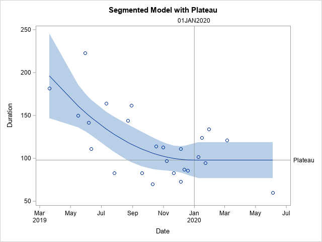
It fits a quadratic, and then plateaus after a particular breakpoint. For theory testing I imagine the breakpoint itself will be of interest to many criminologists, and you can estimate that location in this formulation.

Rick works for SAS, and so if familiar with SAS go ahead and use his code. But here I coded up an example fitting a constrained non-linear regression in python using scipy.

Python Code

Taking the same data from Rick Wicklin’s blog post, this code just reads in the data and converts dates to days since 3/20/2019. I don’t scale the data here to be an exact replicate of Rick’s blog post, but for data with a wider range it would be necessary to prevent some numerical instability.

# Python libraries to replicate

from datetime import datetime
import numpy as np
import pandas as pd
from scipy.optimize import minimize
from scipy.optimize import NonlinearConstraint

# Via https://blogs.sas.com/content/iml/2020/12/14/segmented-regression-sas.html
dat = [(1,'3/20/2019',182),
       (3,'5/30/2019',223),
       (5,'6/11/2019',111),
       (7,'7/26/2019',83),
       (9,'8/29/2019',162),
       (11,'10/10/2019',70),
       (13,'10/31/2019',113),
       (15,'11/21/2019',83),
       (17,'12/5/2019',73),
       (19,'12/19/2019',86),
       (21,'1/16/2020',124),
       (23,'1/30/2020',134),
       (25,'6/4/2020',60),
       (2,'5/16/2019',150),
       (4,'6/6/2019',142),
       (6,'7/11/2019',164),
       (8,'8/22/2019',144),
       (10,'9/19/2019',83),
       (12,'10/17/2019',114),
       (14,'11/7/2019',97),
       (16,'12/5/2019',111),
       (18,'12/12/2019',87),
       (20,'1/9/2020',102),
       (22,'1/23/2020',95),
       (24,'3/5/2020',121)]

df = pd.DataFrame(dat,columns=['SugeryNo','Date','Duration'])
df['Date'] = pd.to_datetime(df['Date'])
df['DaysRef'] = (df['Date'] - pd.to_datetime('3/20/2019')).dt.days
df['DR2'] = df['DaysRef']**2

Now, one of the things I sometimes find confusing in posts that optimize arbitrary functions (in R or python) is that to minimize a function, it is with respect to your data at hand. Sometimes folks have functions that can pass in data and the parameters. But I find it easier to just keep the data fixed and only pass in parameters.

So you can see in my non-linear pred function, it passes in the parameters (which we will estimate), and gives a prediction for the fixed dataset. Ditto for the loss function (you could update to do logistic regression for example if predicting 0/1s). Then the nlconst object is a special python function to define the non-linear constraints that make this plateau model work. Then start solutions and finally minimize the function (using a Fortran solver!):

# Pass in global data into the function
def prednl(x):
    b0 = x[0]
    b1 = x[1]
    b2 = x[2]
    brp = x[3]
    before = (df['DaysRef'] < brp)
    y0 = b0 + b1*df['DaysRef'] + b2*df['DR2']
    y1 = b0 + b1*brp + b2*brp*brp
    return y0*before + (~before)*y1

def lossnl(x):
    yhat = prednl(x)
    squares = (df['Duration'] - yhat)**2
    return squares.sum()

def nlconst(x):
    r1 = x[4] - (x[0] + x[1]*x[3] + x[2]*x[3]*x[3])    # plateau
    r2 = x[3] - ((-0.5*x[1])/x[2])                     # breakpoint
    # Could also consider bounds on breakpoint and curve needs to be non-zero
    return np.array([r1,r2])

nlc = NonlinearConstraint(nlconst, np.array([0.0,0.0]), 
                                   np.array([0.0,0.0]))

start = np.array([185.0,-1.0,0.1,150.0,60.0])

solution = minimize(lossnl,start,method='trust-constr',
                    constraints=nlc,options={'maxiter':50000})

And this returns the same fit as did the SAS routine:

Now I will admit defeat to trying to figure out analytical standard errors (tried via the outer product gradient approach via autograd, as well as using BFGS and its inverse hessian estimate, which is not even close to the results SAS gives).

So I do the thing all lazy statisticians do at this point – the bootstrap. (SPSS I believe will only give standard errors for its nonlinear estimates via bootstrap.)

# Do the bootstrap, 95% CI
res = []
mess = []
for i in range(19):
    print(f'iter {i+1}: ',datetime.now())
    boot = df.sample(n=df.shape[1],replace=True).reset_index(drop=True)
    days_ref = boot['DaysRef'].to_numpy()
    duration = boot['Duration'].to_numpy()
    dr2 = boot['DR2'].to_numpy()
    def lb(x):
        b0 = x[0]
        b1 = x[1]
        b2 = x[2]
        brp = x[3]
        before = (days_ref < brp)
        y0 = b0 + b1*days_ref + b2*dr2
        y1 = b0 + b1*brp + b2*brp*brp
        yhat = y0*before + (~before)*y1
        squares = (duration - yhat)**2
        return squares.sum()
    sl = minimize(lb,start,method='trust-constr',
                  constraints=nlc,options={'maxiter':50000})
    mess.append(sl.message)
    print(sl.message)
    res.append(sl.x)

rdf = pd.DataFrame(res,columns=['B0','B1','B2','break','plateau'])
rdf.describe() #min/max are the 95% CIs

And we can see that these estimates are very wide. We can look at individual iterations, and in a few the estimates go off the rails (and they still say they converged, they just converged to non-sense).

# Some of the wayward estimates
# still pass convergence
rdf['Eval'] = mess
rdf

But this is the nature of these non-linear functions. They can be pretty finicky. If a straight line fits the data quite well, the quadratic term will be very small, and so the estimated plateau may be outside of the data (or just totally unstable).

Still, even though it is more work and potentially more finicky in model fitting, I would rather people have explicit functional form predictions for non-linear effects, than simply throwing in polynomial functions and writing a paper about “look at these non-linear effects”.

And this formulation provides an explicit mechanism to measure the location of a plateau effect directly as a parameter.