本文使用的工具为MATLAB以及Peter Corke的RTB(Robotics Toolbox)。基于RTB 10.3.1版本，我写了RTE(Robotics Toolbox Extension)，增加了一些移动机器人、机械臂以及路径规划相关代码。同时，RTE也修复了原RTB的一些小bug。

听说最近RTB出了10.4，不知道bug修复完没有，有用过的同学可以谈谈感想。个人建议这篇文章最好用我GitHub里的RTE工具箱，下载点这里。安装方法见README文件，写的很详细了。

本文的任务是利用MATLAB和RTB建模二连杆机械臂的动力学，并与MATLAB自带的simulink/simscape仿真进行对比，验证RTB建模的正确性。本文并不涉及控制部分，只是教大家如何建模真实的多刚体系统。

二连杆机械臂

如图1所示，我们要研究的是竖直平面上的二连杆机械臂，也可以说是双摆。因为本文不做控制，所以我们要模拟机械臂在重力的作用下运动的过程。

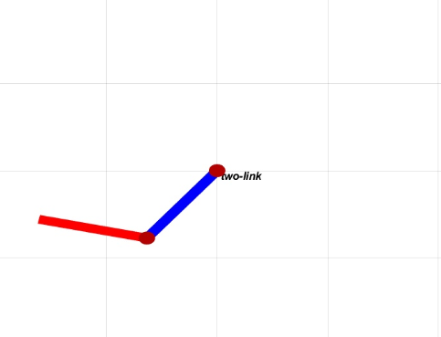
图1. 竖直平面上的二连杆机械臂

这里给出二连杆机械臂的动力学建模过程[1]，之后可以代入数值验证代码正确性。

机械臂的动能为

T(θ,θ˙)=12m1∥v1∥2+12ω1TI1ω1+12m2∥v2∥2+12ω2TI2ω2，(1)T(\theta,\dot \theta)=\frac{1}{2}m_1\|v_1\|^2+\frac{1}{2}\omega_1^T\mathcal I_1\omega_1+\frac{1}{2}m_2\|v_2\|^2+\frac{1}{2}\omega_2^T\mathcal I_2\omega_2，\qquad(1) T(θ,θ˙)=21​m1​∥v1​∥2+21​ω1T​I1​ω1​+21​m2​∥v2​∥2+21​ω2T​I2​ω2​，(1)

其中，I1\mathcal I_1I1​，I2\mathcal I_2I2​是关于质心的转动惯量。

分析各连杆关于质心的位置和速度为

xˉ1=r1c1xˉ1˙=−r1s1θ˙1yˉ1=r1s1xˉ1˙=r1c1θ˙1xˉ2=l1c1+r2c12xˉ2˙=−(l1s1+r2s12)θ˙1−r2s12θ˙2yˉ1=l1s1+r2s12xˉ1˙=(l1c1+r2c12)θ˙1+r2c12θ˙2\begin{aligned} \bar x_1&=r_1c_1&\dot {\bar x_1}&=-r_1s_1\dot \theta_1\\ \bar y_1&=r_1s_1&\dot {\bar x_1}&=r_1c_1\dot \theta_1\\ \bar x_2&=l_1c_1+r_2c_{12}&\dot {\bar x_2}&=-(l_1s_1+r_2s_{12})\dot \theta_1-r_2s_{12}\dot \theta_2\\ \bar y_1&=l_1s_1+r_2s_{12}&\dot {\bar x_1}&=(l_1c_1+r_2c_{12})\dot \theta_1+r_2c_{12}\dot \theta_2 \end{aligned} xˉ1​yˉ​1​xˉ2​yˉ​1​​=r1​c1​=r1​s1​=l1​c1​+r2​c12​=l1​s1​+r2​s12​​xˉ1​˙​xˉ1​˙​xˉ2​˙​xˉ1​˙​​=−r1​s1​θ˙1​=r1​c1​θ˙1​=−(l1​s1​+r2​s12​)θ˙1​−r2​s12​θ˙2​=(l1​c1​+r2​c12​)θ˙1​+r2​c12​θ˙2​​

其中，r1r_1r1​，r2r_2r2​是关节离重心的距离。代入式1得，

T(θ,θ˙)=12[θ˙1θ˙2]T[α+2βc2δ+βc2δ+βc2δ][θ˙1θ˙2]，T(\theta,\dot \theta)=\frac{1}{2}\begin{bmatrix} \dot \theta_1\\ \dot \theta_2 \end{bmatrix}^T\begin{bmatrix} \alpha+2\beta c_2&\delta+\beta c_2\\ \delta+\beta c_2&\delta \end{bmatrix}\begin{bmatrix} \dot \theta_1\\ \dot \theta_2 \end{bmatrix}， T(θ,θ˙)=21​[θ˙1​θ˙2​​]T[α+2βc2​δ+βc2​​δ+βc2​δ​][θ˙1​θ˙2​​]，

α=Iz1+Iz2+m1r12+m2(l12+r22)β=m2l1r2δ=Iz2+m2r22。\begin{aligned} \alpha&=\mathcal I_{z1}+\mathcal I_{z2}+m_1r_1^2+m_2(l_1^2+r_2^2)\\ \beta&=m_2l_1r_2\\ \delta&=\mathcal I_{z2}+m_2r_2^2。 \end{aligned} αβδ​=Iz1​+Iz2​+m1​r12​+m2​(l12​+r22​)=m2​l1​r2​=Iz2​+m2​r22​。​

参考我之前柔性机械臂建模的文章中的拉格朗日运动方程，可得

ddt∂T∂θ˙=[α+2βc2δ+βc2δ+βc2δ][θ¨1θ¨2]+[−2βs2θ˙2−βs2θ˙2−βs2θ˙20][θ˙1θ˙2]，∂T∂θ=[0−(βs2θ˙12+βs2θ˙1θ˙2)]=[−βs2θ˙2βs2θ˙1−βs2(θ˙1+θ˙2)0][θ˙1θ˙2]。\begin{aligned} \frac{d}{dt}\frac{\partial T}{\partial \dot \theta}&=\begin{bmatrix} \alpha+2\beta c_2&\delta +\beta c_2\\ \delta+\beta c_2&\delta \end{bmatrix}\begin{bmatrix} \ddot \theta_1\\ \ddot \theta_2 \end{bmatrix}+\begin{bmatrix} -2\beta s_2\dot \theta_2&-\beta s_2\dot \theta_2\\ -\beta s_2\dot \theta_2&0 \end{bmatrix}\begin{bmatrix} \dot \theta_1\\ \dot \theta_2 \end{bmatrix}，\\ \frac{\partial T}{\partial \theta}&=\begin{bmatrix} 0\\ -(\beta s_2\dot \theta_1^2+\beta s_2 \dot \theta_1\dot \theta_2) \end{bmatrix} =\begin{bmatrix} -\beta s_2\dot \theta_2&\beta s_2\dot \theta_1\\ -\beta s_2(\dot \theta_1+ \dot \theta_2)&0 \end{bmatrix}\begin{bmatrix} \dot \theta_1\\ \dot \theta_2 \end{bmatrix}。 \end{aligned} dtd​∂θ˙∂T​∂θ∂T​​=[α+2βc2​δ+βc2​​δ+βc2​δ​][θ¨1​θ¨2​​]+[−2βs2​θ˙2​−βs2​θ˙2​​−βs2​θ˙2​0​][θ˙1​θ˙2​​]，=[0−(βs2​θ˙12​+βs2​θ˙1​θ˙2​)​]=[−βs2​θ˙2​−βs2​(θ˙1​+θ˙2​)​βs2​θ˙1​0​][θ˙1​θ˙2​​]。​

上面这第二步推导是真的难，我想了好久才想出来，这说明哥氏力其实表达方式不唯一。
两式相减得到

[α+2βc2δ+βc2δ+βc2δ][θ¨1θ¨2]+[−βs2θ˙2−βs2(θ˙1+θ˙2)βs2θ˙10][θ˙1θ˙2]=[τ1τ2]\begin{bmatrix} \alpha+2\beta c_2&\delta +\beta c_2\\ \delta+\beta c_2&\delta \end{bmatrix}\begin{bmatrix} \ddot \theta_1\\ \ddot \theta_2 \end{bmatrix}+\begin{bmatrix} -\beta s_2\dot \theta_2&-\beta s_2(\dot \theta_1+ \dot \theta_2)\\ \beta s_2\dot \theta_1&0 \end{bmatrix}\begin{bmatrix} \dot \theta_1\\ \dot \theta_2 \end{bmatrix}=\begin{bmatrix} \tau_1\\ \tau_2 \end{bmatrix} [α+2βc2​δ+βc2​​δ+βc2​δ​][θ¨1​θ¨2​​]+[−βs2​θ˙2​βs2​θ˙1​​−βs2​(θ˙1​+θ˙2​)0​][θ˙1​θ˙2​​]=[τ1​τ2​​]

重力和摩擦力很简单，它们都只与θ\thetaθ相关，与θ˙\dot \thetaθ˙无关，这里就省略了。

RTB建模

• 给出物理参数

lx = 1; lr = 0.1;  % 连杆的长度和半径
gy = 9.81;  % 重力加速度(这里在y轴方向，因为z轴是关节转动轴)
fvis = 0; fcou = 0; % 粘性摩擦系数和库伦摩擦系数

• 建立连杆模型
  这里的Cuboid和Cylinder都是我自己基于RTB写的类。

rod = Cuboid([lx,lr,lr]); % 建立成长方体
Irod = rod.inertia; % 可以直接获得转动惯量

这里建立成圆柱也行，获得转动惯量时需要进行一个刚体变换。

rod = Cylinder(lr,lx);
Rcyl = SO3.rpy([0 -pi/2 0]);
Irod = Rcyl.R*rod.inertia*Rcyl.R';

• 机械臂建模

% 设定dh参数，质量，关节质心距离，关节约束，转动惯量，摩擦系数
dpm = {'a', lx, 'm', rod.mass, 'r', [-lx/2,0,0],...
 'qlim', [-pi/2, pi/2],'I', Irod,...
    'B', fvis, 'Tc', [fcou -fcou]};
% 建立二连杆机械臂，设定回转关节和重力
r = SerialLink([Revolute(dpm{:}),Revolute(dpm{:})],...
'name','two-link','gravity',[0 gy 0]);

经过以上步骤，二连杆机械臂建模完成，设置关节角qz，可以画出机械臂，效果如图1所示。

ws = [-4 4 -4 4 -4 4]; % 设置工作空间
plotopt = {'workspace', ws, 'nobase', 'notiles', 'noshading', 'noshadow', 'nowrist','top'}; % 设置绘图参数
h = r.plot(qz,plotopt{:});

仿真与验证

我们这里验证二连杆机械臂在重力作用下运动过程，即双摆实验。

% 给定初始关节角位置和速度
qz = zeros(1,2);
qd = zeros(1,2);
% 设定仿真时间10s
y0 = [qz,qd]'; tspan = [0 10]; 
% 刚体仿真用ode15s比较快，用accel函数直接获得关节加速度
tic
[tlist,ylist] = ode15s(@(t,y) [y(r.n+1:end);r.accel(y(1:r.n)',y(r.n+1:end)',zeros(1,r.n))],tspan,y0);
toc
% 差不多6s可出结果，然后画出机械臂即可
ws = [-4 4 -4 4 -4 4];
plotopt = {'workspace', ws, 'nobase', 'notiles', 'noshading', 'noshadow', 'nowrist','top'};
h = r.plot(ylist(:,1:r.n),plotopt{:});

实验结果如下图所示。

下面进行simulink/simscape的双摆仿真，对比实验如下图所示，可以看到前面几乎是同步的。

如何使用simscape搭建一个双摆系统，可以参考b站这个视频。

本文所需全部源代码已上传至我的GitHub，点击这里下载。运行two_link_test.m即可。使用前请确认RTB已经正确安装，下载和安装说明点击这里。

使用simulink/simscape做的双摆仿真也在该仓库里，见link_test.slx，但是需要MATLAB里有simscape的工具箱，否则打不开。另外MATLAB版本最好在2018b以上。

如果喜欢，欢迎点赞和fork。

1. Murray, R. M. (1994). A mathematical introduction to robotic manipulation. CRC press. ↩︎