Baldur's Gate: Multinomial Edition

In a brief bout of escapism from the world and responsibilities, I booted up Baldur’s Gate 2 with my brother. It’s an amazing game, once you have figured out how to roll your character.

For today’s installment; rather than telling you about the game, let’s talk about the maths behind rolling a 2e character for BG2, and then running simulations with weird X-based linux tools.

Rolling a character

The BG2 character generation mechanics is almost entirely based on the rules from AD&D 2e. You get 6 ability scores, and each ability score is rolled as the sum of 3d6.

Probablistically; this should give you a character with an expected 63 total ability points (as a result of rolling 18d6).

Mechanically, you are in this screen:

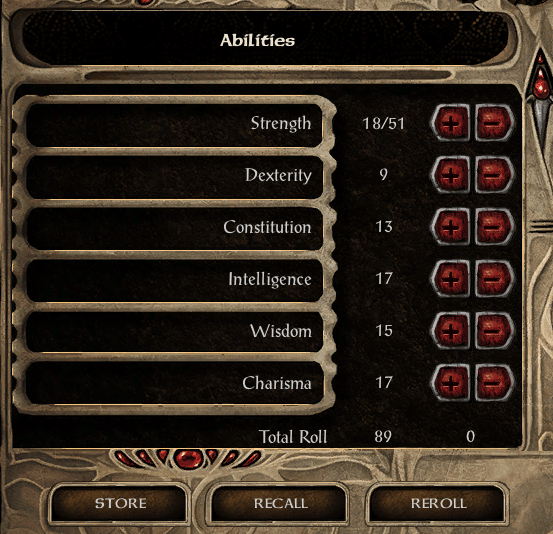
…and they have given you a reroll button.

It’s a strange design idea to port the rolling mechanics from d&d into this game. In a normal campaign you’d usually get one chance rolling, but here, there’s no downside to keeping going; encouraging excessive time investment (the irony in writing a blog post on this is not lost on me). The character creation in BG2 would probably have been less perfection focused if they’d gone for something like 5e point buy.

Anyway, suppose you want learn how to automate this, or you just want to think about combinatorics, multinomials, and weird X tools for a while, then this is the right place. You will also figure out how long it’s expected to take to roll high.

HINT: ..it’s less time than it took to write this blogpost

Disclaimer

Using the script used herein to achieve higher rolls than you have patience for, is on some level; cheating. That said, it’s a fairly pointless effort:

• this is an old, unranked rpg with difficulty settings
• having dump stats is not heavily penalized in the game
• early items nullify effects of common dump stats (19 STR girdle or 18 CHA ring)
• you can get max stats in 20 minutes with by abusing inventory+stat underflow
• some NPCS come with gear that blows marginally better stats out of the water

So assuming you have a reason to be here despite this; let’s dive in to some maths.

Multinomials and probabilities

How likely are you to get a 90/95/100?

The sum of rolling 18 six-sided dice follows an easier variant of the multinomial distribution where we have equal event probabilities. We are going to follow the simpler multinomial expansion from mathworld/Dice for s=6 and n=18 and find P(x,18,6)P(x, 18, 6)P(x,18,6) which we will denote as P(X=x)P(X = x)P(X=x); the chance of rolling a sum equal to xxx:

P(X=x)=1618∑k=0⌊(x−18)/6⌋(−1)k(18k)(x−6k−117)P(X = x) = \frac{1}{6^{18}} \sum_{k=0}^{\lfloor(x-18)/6\rfloor} (-1)^k \binom{18}{k} \binom{x-6k-1}{17}P(X=x)=6181​k=0∑⌊(x−18)/6⌋​(−1)k(k18​)(17x−6k−1​) =∑k=0⌊(x−18)/6⌋(−1)k18k!(18−k)!(x−6k−1)!(x−6k−18)! = \sum_{k=0}^{\lfloor(x-18)/6\rfloor} (-1)^k \frac{18}{k!(18-k)!} \frac{(x-6k-1)!}{(x-6k-18)!}=k=0∑⌊(x−18)/6⌋​(−1)kk!(18−k)!18​(x−6k−18)!(x−6k−1)!​

If we were to expand this expression, we would get 15 different expressions depending on how big of an xxx you want to determine. So rather than trying to reduce this to a polynomial expression over ppp, we will paste values into wolfram alpha and tabulate for [18,…,108][18, \ldots, 108][18,…,108].

You can see the appendix for the numbers. Here we will just plot the values:

and with the precise distribution we can also calculation expectation and variance:

• E(X)=63E(X) = 63E(X)=63
• Var(X)=52.5≈7.242Var(X) = 52.5 \thickapprox 7.24^2Var(X)=52.5≈7.242

This is how things should look on paper. From the chart you can extract:

• 108 would be a once in 101 trillion (6186^{18}618) event
• 107 would be a once in 5 trillion event (6^18/18)
• 106 would be a once in 600 billion event (5s in two places, or 4 in one place)
• 105 would be a once in 90 billion event (3x5s, or 1x4 and 1x5, or 1x3)
• 104 would be a once in 16 billion event (4x5s, 2x5s and 1x4, 2x4s, 1x5 and 1x3, 1x2)
• 103 would be a once in 4 billion event (…)
• 102 would be a once in 1 billion event
• 101 would be a once in 290 million event
• 100 would be a once in 94 million event
• 99 would be a once in 32 million event
• …\ldots…
• 95 would be a once in 900k event (first number with prob < 1 in a million)

But is this really right for BG? A lot of people have all rolled nineties in just a few hundred rolls, and many even getting 100 or more..was that extreme luck, or are higher numbers more likely than what this distribution says?

Well, let’s start with the obvious:

The distribution is censored. We don’t see the rolls below 757575.

What’s left of this cutoff actually accounts for around 94% of the distribution. If the game did not do this, you’d be as likely getting 36 as a 90. We are effectively throwing away “19 bad rolls” on every roll.

AD&D 2e had its own ways to tilt the distribution in a way that resulted in more powerful characters.

How such a truncation or censoring is performed is at the mercy of the BG engine. We will rectify the distribution by scaling up the truncated version of our distribution, and show that this is correct later.

Here we have divided by the sum of the probabilities of the right hand side of the graph P(X≥75)P(X \ge 75)P(X≥75) to get the new probability sum to 1.

Using this scaled data, we can get precise, truncated distribution parameters:

• E(XT)=77.525E(X_T) = 77.525E(XT​)=77.525
• Var(XT)=2.612Var(X_T) = 2.61^2Var(XT​)=2.612

This censored 18d6 multinomial distribution is actually very close for certain cases, and we will demonstrate this.

But first, we are going to need to press the reroll button a lot…

Automating Rolling

The simulation script / hacks we made is found here.

Tools

We are playing on Linux with X and some obscure associated tooling:

• scrot - X screenshot utility
• xdotool - X CLI automation tool
• xwininfo - X window information utility

Basic strategy;

• find out where buttons are with xwininfo
• press the reroll button with xdotool
• take screenshot of the total number with scrot
• compare screenshot to previous rolls
• press store when a new maximum is found

The script also does some extra stuff to determine the strength roll, but that’s not relevant here.

Initialization

To standardise what we are taking screenshots of, we need a consistent frame of reference.

xwininfo will give us the x,y coordinates of the top left corner of the game window, and then hard-code the offsets from that because the game has a consistent layout. There is some complexity in doing this, but it has so far worked well.

Caveat: You need to have scaled the window to size >= 1024x768 to avoid UI downscaling.

The standardised approach also helps with dealing with rolls, and it let us populate a roll-table quickly.

Roll Tables

Taking screenshots is pretty easy. Use scrot at an x,y coordinate followed by lenghts; ,width,height as remaining arguments defining the square to screenshot:

scrot -a "${STR_TOP_LEFT_X},${STR_TOP_LEFT_Y},49,17" -

the output of this can be piped to a .png and passed to compare (part of imagemagick package), to compare values based on thresholds. However, this idea is actually overkill..

The menu background is static and the resulting screenshots are actually completely deterministic per value, so we can instead just compare them by their hashes in one big switch (i.e. after piping to md5) and use that as our roll table, Excerpt:

    d74939b47327e4f2c1b781d64e2ab28d*) CURRENT_ROLL=90 ;;
    ca49ce8b4c9c0f814dab24668f7313fe*) CURRENT_ROLL=91 ;;
    3e6f8127ac0634bb1fc20acf40c95c48*) CURRENT_ROLL=92 ;;
    7f849edd84a4be895f5c58b4f5b20d4e*) CURRENT_ROLL=93 ;;
    b8f90179e2a0e975fc2647bc7439d9c6*) CURRENT_ROLL=94 ;;
    b1d3b73de16d750b265f5c63000ccd54*) CURRENT_ROLL=95 ;;
    87413f7310bd06b0b66fb4d2e61c5c7a*) CURRENT_ROLL=96 ;;
    b489ad2a17456f8eebe843e4b7e3e685*) CURRENT_ROLL=97 ;;
    25112e67464791f24f9e2e99d38ef9d7*) CURRENT_ROLL=98 ;;
    9c3720b9d3ab1d7f0d11dfb9771a1aef*) CURRENT_ROLL=99 ;;
    3ef9bf6cd4d9946d89765870e5b21566*) CURRENT_ROLL=100 ;;

Clicking

Automating a click is simply:

xdotool mousemove "$REROLL_BTN_X" "$REROLL_BTN_Y" click --delay=0 1

where the --delay=0 overrides a builtin delay between clicks.

The only complication here is that BG performs internal buffering of clicks, so this allows us to blast through numbers faster than the screen can display them. This means we have to compensate with a sleep 0.001 after clicking to ensure we can grab the scrot of the roll before another click is registered.

Showcase

Running the script (with a terminal showing the script output overlayed) looks like this:

On my machine, we get just over 15 rolls per second.

Sampling

We rolled a human fighter, paladin, and a ranger overnight with roughly half a million rolls each (see appendix), and we got these values:

Let’s start with the fighter. If we compare the fighter graph with our precise, censored multinomial distribution, they are very close:

So for fighters, we can be pretty happy with the calculations we have done, and can use the precise probabilities as a guide.

How long would it take you to achieve >95 for a fighter using the script?

• 108 is a once in 5 trillion event (10,000 years)
• 107 is a once in 300 billion event (600 years)
• 106 is a once in 33 billion event (69 years)
• 105 is a once in 5 billion event (10 years)
• 104 is a once in 900 million event (2 years)
• 103 is a once in 200 million event (5 months)
• 102 is a once in 50 million event (5 weeks)
• 101 is a once in 16 million event (2 weeks)
• 100 is a once in 5 million event (4 days)
• 99 is a once in 2 million event (1.5 day)
• 98 is a once in 700k event (12h)
• 97 is a once in 270k event (5h)
• 96 is a once in 110k event (2h)
• 95 is a once in 50k event (55m)

So if we only look at human fighters or mages, we can stop here:

We are actually quite a lot more likely to get a good roll early than what just the pure dice math would indicate thanks to censoring (50k rolls => likely 95 rather than estimated 90 without censoring).

However, what’s up with the paladins and rangers? Time for a more painful math detour.

Class/Race Variance

The reason for the discrepancy is simple: stat floors based on races/class.

These stat floors are insignificant in some cases, but highly significant in others. Some highly floored classes actually push the uncensored mean above the 75 cutoff even though it’s a whole 12 points above the mean of the original underlying distribution.

The floors for a some of the classes:

• fighter mins: STR=9, rest 3
• mage mins: INT=9, rest 3
• paladin mins: CHA=17, WIS=13, STR=12, CON=9, rest 3
• ranger mins: CON=14, WIS=14, STR=13, DEX=13, rest 3
• other classes mins: generally light floors

In other words: paladins and rangers have significantly higher rolls on average.

Sidenote: in 2e you actually rolled stats first, and only if you met the requirements could you become a Paladin / Ranger. It’s an interesting choice. Would not call this fun.

Anyway. Is it possible to incorporate these floors into our modelling?

Floored Ability Distributions

If floors are involved at earlier stages, we have to take a step back and look at the distributions that make up the sum. We can compute distributions for individual ability scores (even if floored) if we use the distribution for P(x,3,6)P(x, 3, 6)P(x,3,6) from mathworld/Dice where s=6 and n=3 and censor it at a cutoff point similar to how we censor the total distribution.

Computing the value without a floor follows the same setup as when we did 18 dice; use wolfram alpha and tabulate for [3,…,18][3, \ldots, 18][3,…,18]:

then we truncate + scale this at the observed floor points 9, 12, 13, 14, and 17:

To avoid having to write out conditionals P(X=x∣X≥k)P(X = x| X\ge k)P(X=x∣X≥k) everywhere we will denote X⌊k⌋X^{\lfloor k \rfloor}X⌊k⌋ as one of these graphed multinomial distributions for the sum of 3d6 floored at kkk:

X⌊k⌋∼M⌊k⌋(3d6)X^{\lfloor k \rfloor} \sim \mathcal{M}^{\lfloor k \rfloor}(3d6)X⌊k⌋∼M⌊k⌋(3d6)

Note also that an unfloored ability score XXX is equal to X⌊3⌋X^{\lfloor3\rfloor}X⌊3⌋.

We can then compute precise conditional expectations by floor:

• E(X⌊3⌋)=E(X)=3∑k=16k6=3∗3.5=10.5\mathbb{E}(X^{\lfloor3\rfloor}) = \mathbb{E}(X) = 3\sum_{k=1}^{6}\frac{k}{6} = 3*3.5 = 10.5E(X⌊3⌋)=E(X)=3∑k=16​6k​=3∗3.5=10.5
• E(X⌊9⌋)=11.8125\mathbb{E}(X^{\lfloor9\rfloor}) = 11.8125E(X⌊9⌋)=11.8125
• E(X⌊12⌋)=13.5555\mathbb{E}(X^{\lfloor12\rfloor}) = 13.5555E(X⌊12⌋)=13.5555
• E(X⌊13⌋)=14.2500\mathbb{E}(X^{\lfloor13\rfloor}) = 14.2500E(X⌊13⌋)=14.2500
• E(X⌊14⌋)=15.0000\mathbb{E}(X^{\lfloor14\rfloor}) = 15.0000E(X⌊14⌋)=15.0000
• E(X⌊17⌋)=17.2500\mathbb{E}(X^{\lfloor17\rfloor}) = 17.2500E(X⌊17⌋)=17.2500

Similarly, we can compute precise variances:

• Var(X⌊3⌋)=Var(X)=3∑k=16(xi−3.5)26=3∗2.92=8.75Var(X^{\lfloor3\rfloor}) = Var(X) = 3\sum_{k=1}^6\frac{(x_i - 3.5)^2}{6} = 3*2.92 = 8.75Var(X⌊3⌋)=Var(X)=3∑k=16​6(xi​−3.5)2​=3∗2.92=8.75
• Var(X⌊9⌋)=4.5773Var(X^{\lfloor9\rfloor}) = 4.5773Var(X⌊9⌋)=4.5773
• Var(X⌊12⌋)=2.2469Var(X^{\lfloor12\rfloor}) = 2.2469Var(X⌊12⌋)=2.2469
• Var(X⌊13⌋)=1.6875Var(X^{\lfloor13\rfloor}) = 1.6875Var(X⌊13⌋)=1.6875
• Var(X⌊14⌋)=1.2000Var(X^{\lfloor14\rfloor}) = 1.2000Var(X⌊14⌋)=1.2000
• Var(X⌊17⌋)=0.1875Var(X^{\lfloor17\rfloor}) = 0.1875Var(X⌊17⌋)=0.1875

Sum of Floored Ability Distributions

Define ZpaladinZ_{paladin}Zpaladin​, ZrangerZ_{ranger}Zranger​ and ZfighterZ_{fighter}Zfighter​ as:

Zpaladin=X1⌊17⌋+X2⌊13⌋+X3⌊12⌋+X4⌊9⌋+X5⌊3⌋+X6⌊3⌋Z_{paladin} = X_1^{\lfloor17\rfloor} + X_2^{\lfloor13\rfloor} + X_3^{\lfloor12\rfloor} + X_4^{\lfloor9\rfloor} + X_5^{\lfloor3\rfloor} + X_6^{\lfloor3\rfloor}Zpaladin​=X1⌊17⌋​+X2⌊13⌋​+X3⌊12⌋​+X4⌊9⌋​+X5⌊3⌋​+X6⌊3⌋​ Zranger=X1⌊14⌋+X2⌊14⌋+X3⌊13⌋+X4⌊13⌋+X5⌊3⌋+X6⌊3⌋Z_{ranger} = X_1^{\lfloor14\rfloor} + X_2^{\lfloor14\rfloor} + X_3^{\lfloor13\rfloor} + X_4^{\lfloor13\rfloor} + X_5^{\lfloor3\rfloor} + X_6^{\lfloor3\rfloor}Zranger​=X1⌊14⌋​+X2⌊14⌋​+X3⌊13⌋​+X4⌊13⌋​+X5⌊3⌋​+X6⌊3⌋​ Zfighter=X1⌊9⌋+X2⌊3⌋+X3⌊3⌋+X4⌊3⌋+X5⌊3⌋+X6⌊3⌋Z_{fighter} = X_1^{\lfloor9\rfloor} + X_2^{\lfloor3\rfloor} + X_3^{\lfloor3\rfloor} + X_4^{\lfloor3\rfloor} + X_5^{\lfloor3\rfloor} + X_6^{\lfloor3\rfloor}Zfighter​=X1⌊9⌋​+X2⌊3⌋​+X3⌊3⌋​+X4⌊3⌋​+X5⌊3⌋​+X6⌊3⌋​

for floored 3d6 based random variables Xi⌊N⌋∼M⌊N⌋(3d6)X_i^{\lfloor N \rfloor} \sim \mathcal{M}^{\lfloor N \rfloor}(3d6)Xi⌊N⌋​∼M⌊N⌋(3d6).

Using the computed expectations above to sum across the 6 main stats:

• E(Fighter)=E(X⌊9⌋)+5E(X)=64.31\mathbb{E}(Fighter) = \mathbb{E}(X^{\lfloor9\rfloor}) + 5\mathbb{E}(X) = 64.31E(Fighter)=E(X⌊9⌋)+5E(X)=64.31
• E(Ranger)=2E(X⌊14⌋)+2E(X⌊13⌋)+2E(X)=79.5\mathbb{E}(Ranger) = 2\mathbb{E}(X^{\lfloor14\rfloor}) + 2\mathbb{E}(X^{\lfloor13\rfloor}) + 2\mathbb{E}(X) = 79.5E(Ranger)=2E(X⌊14⌋)+2E(X⌊13⌋)+2E(X)=79.5
• E(Paladin)=E(X⌊17⌋)+E(X⌊13⌋)+E(X⌊12⌋)+E(X⌊9⌋)+2E(X)=77.86\mathbb{E}(Paladin) = \mathbb{E}(X^{\lfloor17\rfloor}) + \mathbb{E}(X^{\lfloor13\rfloor}) + \mathbb{E}(X^{\lfloor12\rfloor}) + \mathbb{E}(X^{\lfloor9\rfloor})+ 2\mathbb{E}(X) = 77.86E(Paladin)=E(X⌊17⌋)+E(X⌊13⌋)+E(X⌊12⌋)+E(X⌊9⌋)+2E(X)=77.86

and similarly for variance:

• Var(Fighter)=Var(X⌊9⌋)+5Var(X)≈6.952Var(Fighter) = Var(X^{\lfloor9\rfloor}) + 5Var(X) \thickapprox 6.95^2Var(Fighter)=Var(X⌊9⌋)+5Var(X)≈6.952
• Var(Ranger)=2Var(X⌊14⌋)+2Var(X⌊13⌋)+2Var(X)≈4.822Var(Ranger) = 2Var(X^{\lfloor14\rfloor}) + 2Var(X^{\lfloor13\rfloor}) + 2Var(X) \thickapprox 4.82^2Var(Ranger)=2Var(X⌊14⌋)+2Var(X⌊13⌋)+2Var(X)≈4.822
• Var(Paladin)=Var(X⌊17⌋)+Var(X⌊13⌋)+Var(X⌊12⌋)+Var(X⌊3⌋)+2Var(X)≈5.122Var(Paladin) = Var(X^{\lfloor17\rfloor}) + Var(X^{\lfloor13\rfloor}) + Var(X^{\lfloor12\rfloor}) + Var(X^{\lfloor3\rfloor})+ 2Var(X) \thickapprox 5.12^2Var(Paladin)=Var(X⌊17⌋)+Var(X⌊13⌋)+Var(X⌊12⌋)+Var(X⌊3⌋)+2Var(X)≈5.122

noting that variables are independent under the observed two stage censoring.

Why can we rely on two stage censoring and their independence? If any of these internal mechanisms used some kind of if condition or min function, it would be immediately obvious from the distribution. The paladin distribution of charisma is clearly a ~1/4 for an 18, and ~3/4 for a 17; it would have been much rarer to see an 18 otherwise.

Thus, the distributions of our classes are based on multinomal-based distributions with the following first moments:

• UncensoredFighter∼M(μ=64.31,σ2=6.952)Uncensored\ Fighter \sim \mathcal{M}(\mu = 64.31, \sigma^2 = 6.95^2)Uncensored Fighter∼M(μ=64.31,σ2=6.952)
• UncensoredRanger∼M(μ=79.5,σ2=4.822)Uncensored\ Ranger \sim \mathcal{M}(\mu = 79.5, \sigma^2 = 4.82^2)Uncensored Ranger∼M(μ=79.5,σ2=4.822)
• UncensoredPaladin∼M(μ=77.86,σ2=5.122)Uncensored\ Paladin \sim \mathcal{M}(\mu = 77.86, \sigma^2 = 5.12^2)Uncensored Paladin∼M(μ=77.86,σ2=5.122)

This is nice as a quick overview of what’s best in the higher ranges, but it’s not very precise. Without the PMF for the sum of our ability scores, it’s hard to give good values for what the truncated version will look like (we are censoring in two stages). In particular, these heavily floored random variables end up giving us quite asymmetrical distributions in the tails.

Class Distributions

Thankfully, it is possible to inductively compute the pmf of ZclassZ_{class}Zclass​ via convolution.

Some internet digging notwithstanding; most answers found online for this required either mathematica functions (that we do not have here in our inlined source), or a slightly more laborious manual convolution. We will follow the inductive convolution approach which we can solve with recursion. Paladin case:

Let X12=X1⌊17⌋+X2⌊13⌋X_{12} = X_1^{\lfloor17\rfloor} + X_2^{\lfloor13\rfloor}X12​=X1⌊17⌋​+X2⌊13⌋​. We can generate values for the pmf pX12p_{X_{12}}pX12​​ for X12X_{12}X12​ via the pmfs pXip_{X_i}pXi​​ for X1⌊17⌋X_1^{\lfloor17\rfloor}X1⌊17⌋​ and X2⌊13⌋X_2^{\lfloor13\rfloor}X2⌊13⌋​ via the convolution formula:

P(X12=n)=(pX1∗pX2)(n)=∑m=−∞∞P(X1=m)P(X2=n−m)P(X_{12} = n) = (p_{X_1} * p_{X_2})(n) = \sum_{m=-\infty}^{\infty}P(X_1=m)P(X_2 = n-m)P(X12​=n)=(pX1​​∗pX2​​)(n)=m=−∞∑∞​P(X1​=m)P(X2​=n−m)

This step is particularly easy for the paladin, because X1⌊17⌋X_1^{\lfloor17\rfloor}X1⌊17⌋​ only takes two values (i.e. m=17m=17m=17 ahd m=18m=18m=18 are the only non-zero parts in the sum).

The rest is less easy to do by hand, as the sums get increasingly large while we iterate towards Z=P123456Z=P_{123456}Z=P123456​ by repeatedly applying convolution to the remaining XiX_iXi​:

P(X123=n)=(pX12∗pX3)(n)∑m=−∞∞P(X12=m)P(X3=n−m)P(X_{123} = n) = (p_{X_{12}} * p_{X_3})(n) \sum_{m=-\infty}^{\infty}P(X_{12}=m)P(X_3 = n-m)P(X123​=n)=(pX12​​∗pX3​​)(n)m=−∞∑∞​P(X12​=m)P(X3​=n−m)

P(X1234=n)=(pX123∗pX4)(n)∑m=−∞∞P(X123=m)P(X4=n−m)P(X_{1234} = n) = (p_{X_{123}} * p_{X_4})(n) \sum_{m=-\infty}^{\infty}P(X_{123}=m)P(X_4 = n-m)P(X1234​=n)=(pX123​​∗pX4​​)(n)m=−∞∑∞​P(X123​=m)P(X4​=n−m)

P(X12345=n)=(pX1234∗pX5)(n)∑m=−∞∞P(X1234=m)P(X5=n−m)P(X_{12345} = n) = (p_{X_{1234}} * p_{X_5})(n) \sum_{m=-\infty}^{\infty}P(X_{1234}=m)P(X_5 = n-m)P(X12345​=n)=(pX1234​​∗pX5​​)(n)m=−∞∑∞​P(X1234​=m)P(X5​=n−m)

P(X123456=n)=(pX12345∗pX5)(n)∑m=−∞∞P(X12345=m)P(X6=n−m)P(X_{123456} = n) = (p_{X_{12345}} * p_{X_5})(n) \sum_{m=-\infty}^{\infty}P(X_{12345}=m)P(X_6 = n-m)P(X123456​=n)=(pX12345​​∗pX5​​)(n)m=−∞∑∞​P(X12345​=m)P(X6​=n−m)

The hard work is correctly matching indexes in our probability arrays that serve as our mass functions to the sum, and defaulting to zero when accessing out of bounds:

// given pXi = [0.75, 0.25], pXj = [0.375, 0.2678, 0.1786, 0.1071, 0.05357, 0.01786]
// (approximations of the first two truncated paladin probability arrays for CHA + WIS)
var convolve = function (pXi, pXj) {
  // pre-allocate a zero-indexed array where our probabilities will go
  var pXij = [...Array(pXi.length + pXj.length - 1).keys()];
  // loop to generate P(Xij = n) for all n
  for (let n = 0; n < pXi.length + pXj.length - 1; n += 1) {
    pXij[n] = 0; // init to zero
    // loop to do sum over m, first variable determines length of this sum
    for (let m = 0; m < pXi.length; m += 1) {
      // we do defaulting outside range with `|| 0`
      pXij[n] += (pXi[m] || 0) * (pXj[n-m] || 0);
    }
  }
  return pXij;
};
// returns [0.28125, 0.29464, 0.2009, 0.125, 0.06696, 0.02678, 0.004464]

Using this, we can compute the PMF for Zclass=X123456Z_{class} = X_{123456}Zclass​=X123456​:

P(Zclass=z)=(((((pX1∗pX2)∗pX3)∗pX4)∗pX5)∗pX6)(z)P(Z_{class} = z) = (((((p_{X_1} * p_{X_2}) * p_{X_3}) * p_{X_4}) * p_{X_5}) * p_{X_6}) (z)P(Zclass​=z)=(((((pX1​​∗pX2​​)∗pX3​​)∗pX4​​)∗pX5​​)∗pX6​​)(z)

and we graph them for various classes:

Notice the heavily tilted ranger/paladin distributions whose lean is distinctively more to the right.

The last thing that’s left now is to rectify ZcZ_cZc​ at 75 to get our true, final distributions:

These match the sampled data almost perfectly as can be seen in more detailed comparisons in the appendix.

As can be seen; ranger is faster at getting high numbers, particularly in the 90 -> 97 range, but if you want rolls >= 100, paladin rolls the highest at the fastest rate.

We end with the expected time to roll above a certain threshold where we use the most efficient class based on the number:

• 108 paladin rolls once in 100 billion ⇒ 210y
• 107 paladin rolls once in 5 billion ⇒ 10y
• 106 paladin rolls once in 600 million ⇒ 1y
• 105 paladin rolls once in 100 million ⇒ 11w
• 104 paladin rolls once in 19 million ⇒ 2w
• 103 paladin rolls once in 5 million ⇒ 4d
• 102 paladin rolls once in 1.4 million ⇒ 1d
• 101 paladin rolls once in 400k ⇒ 7h
• 100 paladin/ranger rolls once in 150k ⇒ 3h
• 99 ranger rolls once in 57k ⇒ 1h
• 98 ranger rolls once in 23k ⇒ 25m
• 97 ranger rolls once in 10k ⇒ 11m
• 96 ranger rolls once in 5k ⇒ 5m
• 95 ranger rolls once in 2k ⇒ 2m

Hope you have enjoyed this random brain dump on probability. Don’t think I have ever been nerd sniped this hard before.. I just wanted to play a game and take a break.

/me closes 20 tabs

Appendix

1. Raw simulation data

2. Tabulated values for 18 dice multinomial probability distribution

3. Tabulated values for 3 dice multinomial probability distribution

3: 1/216
4: 1/72
5: 1/36
6: 5/108
7: 5/72
8: 7/72
9: 25/216
10: 1/8
11: 1/8
12: 25/216
13: 7/72
14: 5/72
15: 5/108
16: 1/36
17: 1/72
18: 1/216

4. Comparing observed vs. computed by class

5. Normal approximations

— eirik ᐸ'⧖ᐳ (@sszynrae) April 7, 2022

See also