A well known way of processing multiple streams of data in parallel is through the use of SIMD instructions. All major chip makers started adding SIMD instructions to their processors in the late 1990s. MMX was added to Intel’s Pentium processor in 1997. It was intended to accelerate image, audio and video processing.

Difference between Single-Instruction-Multiple-Data and Single-Instruction-Single-Data processing.

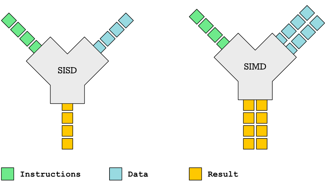
Vector processing is another way of processing multiple streams of data in parallel, but is often thought of as an older more outdated method of doing data parallelism. A reason for this perception is that it was a dominant way of processing data in parallel back in the 1980s on Cray vector processing super computers. When I grew up in the 1980s and early 1990s, Cray was synonymous with supercomputing. I remember fantasizing with my friends about what kind of frame rate we would get running Doom (released 1993) on a Cray computer.

Cray-1 vector processing super computer

However, the fact that vector processing existed and died out before modern SIMD instruction sets gives the wrong idea of the chronology. In computer science, as in fashion, old trends tend to get recycled. SIMD instructions is in fact a much older idea. Sketchpad, widely regarded as the first computer hardware solution with a graphical user interface ran on a Lincoln TX-2 computer which could do SIMD instructions back in 1958. Vector processing machines came much later in the 1970s. Most famous is the Cray-1 released in 1975.

Vector processing is a higher level abstraction. SIMD style processing acts as a more basic building block to construct a vector processor architecture. Now, you may ask if it was a superior system, then why did Cray’s go extinct?

The PC revolution basically killed Cray vector processors. Cray lacked volume. With huge volumes of PCs one could get Cray style computing power by simply using numerous PCs in a cluster. However, today we have reached the end of the road in terms of what you can squeeze out of performance from a general purpose processor.

General purpose processors won over the specialized hardware in the 1980s and 1990s because Moore’s law allowed huge performance increases every year for simple single threaded computation. That world however is long gone. Specialized hardware is back with a vengeance. The only way to boost performance today is through tailor made hardware. That is why Systems-on-a-Chip (SoC) like Apple’s M1 has special hardware for encryption, image processing, neural engines, GPUs and more, all on one and the same silicon die.

The complex processing that once existed only in a Cray super computer can now be built into single silicon dies. Thus it is time to revisit vector processing and try to understand what makes vector processing so powerful compared to the much simpler SIMD style computations. To understand vector processing, we need a grasp of how SIMD instructions work first.

How SIMD Instructions Work

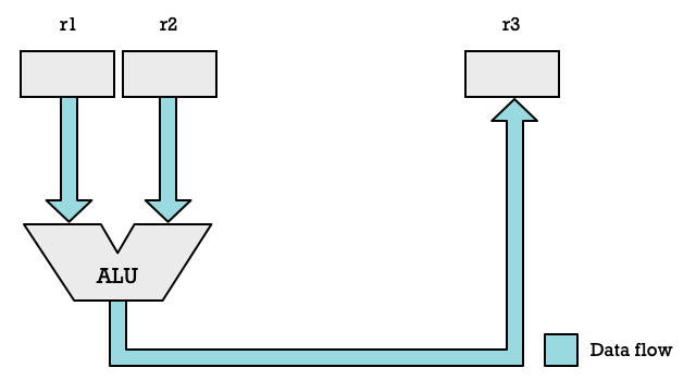
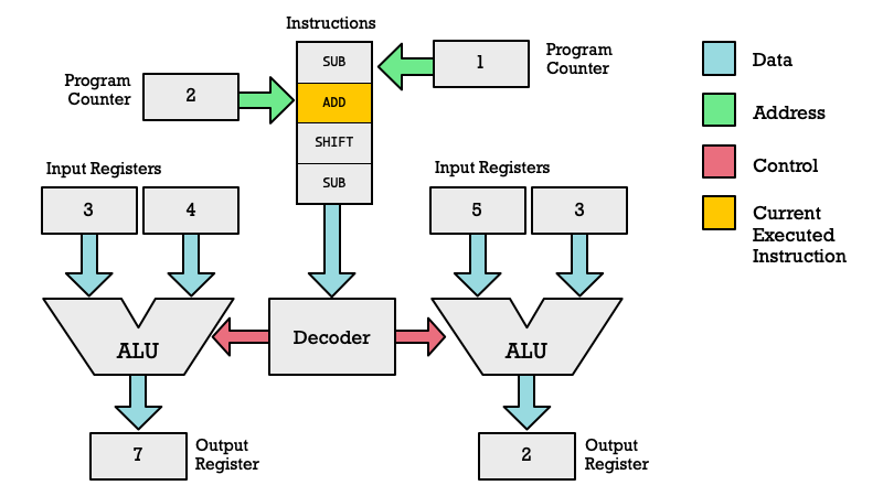
In a simple processor we have registers and the ALU organized as shown in the diagram below. Some register r1 and r2 are used as inputs and the result is stored in another register r2. Of course any register could be used. Depending on the architecture they may be named x0, x1, ..., x31 or they could be r0, r1, ..., r15 as is the case on 32-bit ARM architecture.

Using an Arithmetic Logic Unit (ALU) in SISD fashion.

To support SIMD instruction we add more ALUs to our CPU and segment registers into multiple elements. Thus we could take a 32-bit register and split it into two 16-bit elements which can be fed to a separate ALUs. Now we are suddenly able to double the number of arithmetic operations we are performing each clock cycle.

Using multiple ALUs to allow SIMD processing of data.

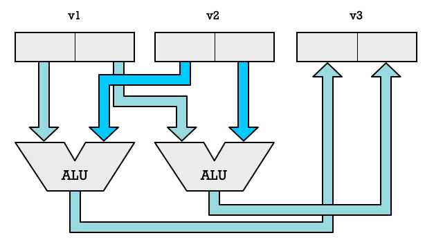
We don’t need to limit ourselves to two ALUs, we could add a lot more. If we have four ALUs we can process four number pairs in parallel. Each element pair combined with an ALU is called a SIMD lane. With two lanes we can process two pairs of numbers. With eight lanes we can process eight numbers in parallel.

How many number we can process in parallel is limited by the length in bits of our general purpose registers or vector registers. On some CPUs you perform SIMD operations on your regular general purpose registers. On others you use special registers for SIMD operations.

But let use RISC-V as an example because it offers a fairly simple instruction-set. We are going to use the ADD16 and ADD8 instructions in the RISC-V P Extension.

The LW (Load Word) instruction will load a 32-bit value on a 32-bit RISC-V processor (RV32IP). We can treat this value as being two 16-bit values and add them up separately. That is what ADD16 does.

# RISC-V Assembly: Add two 16-bit values.

LW    x2, 12(x0)   # x2 ← memory[x0 + 12]
LW    x3, 16(x0)   # x3 ← memory[x0 + 16]
ADD16 x4, x2, x3   
SW    x4, 20(x0)   # x4 → memory[x0 + 20]

As an alternative we could use ADD8 in stead which would treat the 32-bit values we loaded from address 12 and address 16 as four 8-bit values.

# RISC-V Add four 8-bit values.

ADD8  x4, x2, x3

Vector Processing with SIMD Engines

We want to be able to add more SIMD lanes and have larger vector registers. However we cannot do that without adding new instructions when following the packed-SIMD approach.

The solution used by Cray super computers was to define vector-SIMD instructions. With these instructions vector registers are thought of as typeless. The vector instructions don’t say anything about how many elements we have and their size.

This is the strategy used by RISC-V Vector extensions (RVV). With RVV se use an instruction called VSETVLI to configure the size of our elements and number of elements. We fill a register with how many elements we want to process each time we perform a SIMD operation such as VADD.VV (Vector Add with two Vector register arguments).

For instance this instruction tells the CPU to be configured to process 16-bit elements. x2 contains how many elements we want to process. However our SIMD hardware may not have enough large enough registers to process that many 16-bit elements, which is why the instruction will return in x1 the actual number of elements we are able process each time we call a vector-SIMD instruction.

VSETVLI  x1, x2, e16

In practice we have to specify elements size when loading and storing because it influences the ordering of bits. Hence we issue a VLE16.V to load x1 number of 16-bit values. VLSE16.V is used to store x1 number of 16-bit values.

# RISC-V Vector processing (adding two vectors)

VSETVLI  x1, x2, e16 # Use x2 no. 16-bit elements
VLE16.V  v0, (x4)    # Load x1 no. elments into v0
VLE16.V  v1, (x5)    # Load x1 no. elments into v1
VADD.VV  v3, v0, v1  # v3 ← v0 + v1
VLSE16.V v3, (x6)    # v3 → memory[x6]

With vector-SIMD instructions we abstract away how many SIMD lanes we have from the instruction-set. The illustration below shows how vector processing works. Each register has 16 elements, but only two SIMD-lanes. That is not a problem because a vector processor will simply cycle through all the elements until done. In a packed-SIMD we would have processed two pairs of numbers in a clock cycle. With vector-SIMD we spend four CPU clock cycles to get through eight pairs of numbers.

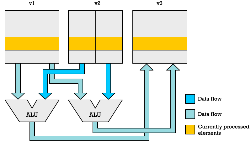
If we had had four SIMD lanes (four ALUs) we could have processed eight pairs of numbers in just two clock cycles. The beauty of this approach is that you can run the exact same code on different CPUs which different number of SIMD lanes.

Thus you could have a cheap microcontroller with just a single-lane or a complex high-end CPU for scientific computing with 64 SIMD-lanes. Both would be able to run the same code. The only difference would be that the high-end CPU would be able to finish faster.

Speeding Up Vector Processing with Pipelining

What I have written about thus far I have covered in various articles in the past. However vector processing contains more tricks to speed up processing beyond what you can achieve with packed-SIMD instructions.

One of the tricks unique to vector processors is pipelining. You may have heard about pipelining in relation to executing regular CPU instructions but this is another form of pipelining. The principle of pipelining is very similar to how modern assembly line manufacturing works. Let me illustrate with examples involving the construction of a robot droid.

We can imagine that there are different workstations named A, B, C and D where different operations and assembly of a robot android is performed. What you will notice here is that while legs are attached at station B, we can see that robot arms get attached at station D. Work on multiple droids is happening in parallel but it is not the same operation performed in parallel.

Pipelined assembly of a droid

We can contrast this interleaving of work with a non-pipelined approach to assembling a robot. Here all assembly is performed on a single droid before a new droid is brought into the assembly line.

Non-pipelined assembly of a droid

There are many examples of using pipelines in the real world. In the grocery store the next customer does not begin processing after the previous one has finished packing their bags. Instead while one customer is paying another one is putting their items on the conveyer belt. In the meantime an earlier customer is packing grocery items into their bag.

Pipelining is exploiting the fact that we don’t need to perform the same tasks and use the same tools all at the same time when building something. In a garage while you are lowering an engine into one car, other workers could be using tools for attaching wheels to another car.

Makers of microprocessor discovered the same opportunities. While one instruction was getting fetched, an earlier instruction could be decoded. While an instruction was getting decoded another one could be executed and so on.

With vector processing we are taking this kind of pipelining thinking further. Consider these simple operations:

# RISC-V Vector processing

VLE32.V   v1, (x1)    # v1 ← memory[x1]
VFMUL.VV  v3, v1, v2  # v3 ← v1 * v2
VFADD.VV  v5, v3, v4  # v5 ← v3 + v4

Say we process vectors with 4 elements and our vector processor only has one lane. In that case we would spend 4 cycles loading all elements into v1, then 4 cycles multiplying v1 with v2 and finally 4 cycles adding v3 to v4. In total we would spend 12 clock cycles.

However vector processing is much faster because while the second element is loaded into v1 we are multiplying the first element loaded on previous clock cycle with the first element of v2. Below you can see an illustration of this process. Instead of consuming 12 clock cycles, we are only spending 6 clock cycles.

Chaining vector operations. Pink outline forms a Convoy

Notice that on the 3rd clock cycles the pipeline is full and we are performing a load, multiplication and addition in parallel. Keep in mind we are doing this on different elements. Each color represents a different element in our vector registers. Blue is the first element in the vector register. Green is the second and so on.

The way this is achieved in vector processing hardware is through something called chaining. Results from one functional unit can be passed directly to the next functional unit without being stored in the vector registers first.

Different functional units such as the Load/Store Unit, Multiplier and Adder (ALU) can be configured to be chained together by the vector processing unit. Conceptually you can imagine an arrangement as seen below. Notice in this example I have reduced the number of vector elements from four to three.

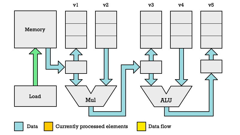
First Clock Cycle

We begin by executing the VLE32.V instruction which takes 3 clock cycles to complete. The Loader specifies a memory location to read (orange arrow) and we pull the data (yellow) out of this memory location.

Please note that this is a gross simplification of how things work. In reality memory reads how higher latency than other operations and will require more clock cycles. Also you don’t read one byte at at time but typically 64 bytes.

However, to grasp the principles of pipelining in a vector processor I am deliberately simplifying.

clock cycle 1 for Loader

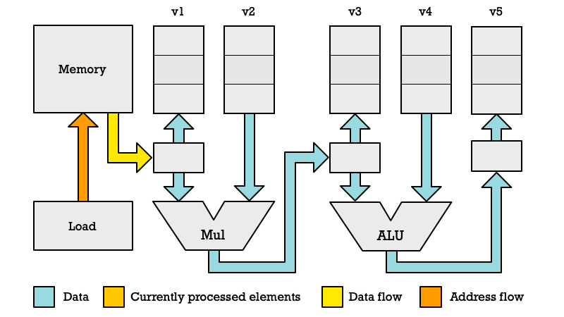
Second Clock Cycle

In the second clock cycle the Loader is loading the second byte. However in this diagram I am showing what is happening in parallel with the Multiplier. While the second element is loaded we are multiplying the first elements of v1 and v2. The first element in v1 isn't being read from that register directly but being chained directly from the loader. We have a register temporarily storing the element previously loaded.

clock cycle 2 for ALU

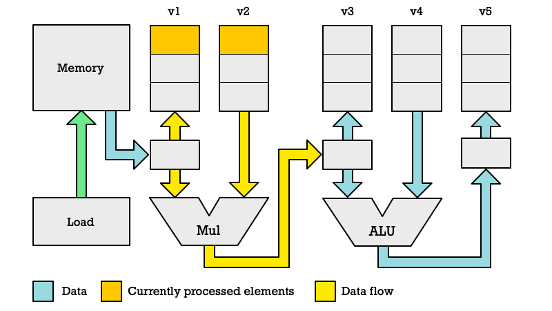
Third Clock Cycle

In the third cycle we are loading the third element from memory, but the diagrams below show what is happening in the Multiplier and the Adder (ALU). The second elements of v1 and v2 get multiplied.

clock cycle 3 for multiplier

In the previous clock cycle we past the product of multiplication as the first argument to the ALU. Thus we add the first element of v4 to the value which was computed by the Multiplier in the previous clock cycle (2nd cycle).

clock cycle 3 for ALU

It should be noted that the diagrams I have made are not ideal. It is hard to draw these things in a sensible way. The way I have drawn it makes it look as if the Loader, Multiplier and Adder are connected in a fixed chain. That is not the case. These computational units can be arranged in any order depending on what instructions are being executed.

What should be the important takeaway is that results from one operation is turned into input for the next operation without a need to read all inputs directly from vector registers.

Convoys of Vector Instructions

You will also note that I have not explained how registers v2 and v4 got their data. These will of course also have to be loaded.

In practice what happens in a vector processor as it reads instructions is that what we call convoys are created. In our example VLE32, FMUL and FADD form a convoy. Instructions in a convoy are executed simultaneously in the same clock cycle.

It is important to note however that the instruction in one convoy are working on different elements. The load instruction VLE32 is loading the 3rd element when the VFMUL is adding the 2nd elements of v1 and v2, while VFADD is adding the 1st elements of v3 and v4.

And to clarify VFADD isn't reading this 1st element directly from v3. It is getting it from the output register of the Multiplier. The inputs of one operation is chained to the outputs of a previous operation.

So as our program is running there will be different convoys forming at different points in time depending on what is possible to run in parallel. In vector processing the time it takes to perform a convoy is called a chime.

You can see from the earlier example how the first convoys will do less work in parallel because we don’t yet have enough data to keep all functional units busy at the same time.

Makeup of convoys

What are the consequences or using convoys for performances? We could measure in clock cycles but given that in real world each vector operation could take multiple clock cycles it would be more accurate to talk about chimes. With 4-element vectors it would take 4 chimes to load all elements. Then another 4 chimes to multiply, then another 4 chimes to add.

4 × 3 = 12  # Chimes when only one operation in each convoy

However we we can see with a pipeline structure where convoys can do multiple operations, you end up with 6 chimes to perform 3 operations on 4 elements.

Superiority of Vector Processing over Array Processing (SIMD)

With packed-SIMD instructions we do array processing. There is no pipelining. We do the same operation on multiple elements each clock cycle. Vector-SIMD instruction in contrast are usually used with vector processing where we use pipelining.

When we add multiple SIMD lanes to a vector processor we get superior performance. Say we have an array processor with 4 SIMD lanes and a vector processor with 4 SIMD lanes each executing the 3 instructions VLE32, VFMUL and VFADD.

An array processor cannot perform the multiply until the load is done. The vector processor in contrast after 3 chimes start performing 3 different operations in parallel, with each operation processing 4 elements. That means in practice you are performing computation on 12 elements in parallel while an array processor (packed-SIMD) would only be doing 4 operations in parallel with the same number of SIMD lanes.

Yet that is only one part of the equation. With vector processor we can have vector registers which are much longer than the number of elements we process each clock cycle. A processor which can do 4 integers in parallel, cannot have more than 128-bit vector registers. A vector processing CPU in contrast could have 1024-bit vector registers without any problems.

With larger vector registers you can process more data before reading the next instruction from the instruction stream. Each vector-SIMD instruction process a lot more elements than a packed-SIMD instruction. That means fewer instructions to decode. More advanced CPUs could use micro-operation caches to alleviate this. However that adds complexity. Vector processing does not require a lot of silicon. That is important because if you can build small cores, it means you can build lots of them which allows you to do more work in parallel.

Advantage of Vector Processing over GPUs

The natural choice for a lot of people today to process large number of elements efficiently is to use GPUs such as Nvidia’s Hopper H100.

Read more:

GPUs are only loosely based on SIMD style processing. A more accurate description is SIMT (Single Instruction Multiple Thread). In this model every SIMD lane works like a thread with its own state, program counter and everything. I will not get into the details of GPU threads, warps and other complexity. You can get some idea of the difference by looking at this diagram of how a GPU core manages two threads (each thread has an ALU). Please note this is a radical simplification, as the real deal would have a numerous different types of computational units to choose from not just ALUs.

Single Instruction Multiple Thread

While a powerful paradigm, it has some major flaws. The architecture came about because GPUs needed to run shader programs. These process each vertex and pixel as a sort of separate thread (SIMD-lane). That is a sensible model for graphics.

However the problem is that GPUs are not general purpose processors. They are not well suited for executing scalar instructions. By that I mean instruction operating on single elements as opposed to multiple elements.

That limitation complicates programming of GPUs. Vector processing can be applied much more easily to scientific computations and machine learning as your compiler has the freedom to mix and match scalar and vector operations. You can also perform regular loops and control flow, which is not something a GPU can do well.

The Future of High Performance Computation

I am a popularizer, so there are many technical aspects I may be missing in my analysis, so verify for yourself if my argumentation makes sense. What I will claim is that vector processing will increasingly displace GPUs for HPC (High performance computation) and Machine Learning. The Fugaku supercomputer for instance is based on many of the same ideas.

Graphics card has a massive head-start in this space because there was money in making really powerful graphics cards for gamers. While graphics cards were not made for general-purpose parallel processing their SIMT style architecture could be adapted for that purpose.

Remember within technology it is not always the best that wins but whomever gets first-mover advantage and reach critical volume. Intel x86 processors were not better than RISC processors in the 1990s but won anyway thanks to higher volume production.

Read more: Why Did Intel x86 Beat RISC Processors in the 1990s?

Companies like Nvidia will surely dominate the field of HPC and Machine Learning for many more years because they have momentum and deep pockets.

Yet I think the vector processing approach will start gaining traction in the peripheral. More machine learning stuff today is getting done outside of data centers on simpler devices. Internet of Things and Edge Computing is an example of that philosophy. You got smart devices connected to the network which collect data and analyze it on the spot rather than sending it across the network to a data center for processing.

Why would you do that? Because the data collected on sight might be a lot and it could be latency sensitive. An obvious example would be self-driving cars collecting video from numerous cameras in addition to LIDAR. Sending all of that data to a datacenter wireless for processing so that the datacenter can send back instructions for which way your car should turn would obviously not be very safe.

Instead you want process data on-site in the car. Thus in the car you have an AI inference engine, meaning a neural network processing inputs and making decisions. However we want to improve and train this neural network model based on collected data. That is why the car will also collect data deemed important and transmit it to a datacenter. Once better AI models have been trained they are transmitted back to the cars at a later stage.

One can imagine that this sort of relation between physical devices out in the real world and data centers will exist for many other types of situations: In factories, stores, power plants, public transportation etc.

With vector processing you can add powerful data processing capability to smart devices while keeping them fairly simple and easy to program. If I add a vector processing extension to a CPU, it is a lot easier to program it than if I add a fancy GPU which requires me to shuffle shader programs and data back and forth between the memory of the CPU and the memory of the GPU.

As RISC-V vector processing gains traction is these kinds of specialized fields and grows in volume I think we will see more of it in areas where GPUs dominate today. The ET-SOC-1 chip from Esperanto Technologies is an example of this kind of strategy. While Esperanto does not use the RISC-V V Extension it does follow the strategy I outlined about using general purpose cores with vector processing capability instead of GPU cores. IEEE Spectrum as an interesting article on this topic for the curious: RISC-V AI Chips Will Be Everywhere.

Let me hear your thoughts. Do you think vector processing has a bright future?