This article builds on Create Your Own Kotlin Playground (and Get a Data Science Head Start) with Jupyter Notebook, which covers the following:

• Jupyter Notebook, an open source web application that lets you create documents that mix text, graphics, and live code. Its native programming language is Python.
• The Kotlin kernel for Jupyter Notebook adds a Kotlin interpreter. The previous article showed how you could use Jupyter Notebook and the Kotlin Kernel as an interactive “playground” for Kotlin code.
• krangl, a library whose name is short for Kotlin library for data wrangling.
• Data frames, which are data structures that represent tables of data organized into rows and columns. They’re the primary data structure in data science applications.

In this article, you’ll take what you’ve learned and build on it by performing basic data science.

Getting Started

If you’re not already running Jupyter Notebook, launch it now. The simplest way to do so is to enter the following on the command line:

jupyter notebook

Your computer will open a new browser window or tab, and it will contain a page that looks similar to this:

Create a new Kotlin notebook by clicking on the New button near the page’s upper right corner. A menu will appear, one of the options will be Kotlin; select that option to create a new Kotlin notebook.

A new browser tab or window will open, containing a page that looks like this:

The page will contain a single cell, a code cell (the default). Enter the following into the cell:

%use krangl

Now run it, either by clicking the Run button or by typing Shift-Enter. This will import krangl.

The cell should look like this for a few seconds…

…then it will look like this:

At this point, krangl should have loaded, and you can now use it for data science.

Working with krangl’s Built-In Data Frames

People who are just getting started with data science often struggle with finding good datasets to work with. To counter this problem, krangl provides three datasets in the form of three built-in DataFrame instances.

Going from smallest to largest, these built-in data frames are:

• sleepData: Data about the sleep patterns of 83 species of animal, including humans.
• irisData: A set of measurements of 150 flowers from different species of iris.
• flightsData: Over 330,000 rows of data about flights taking off from New York City airports in 2013.

Getting a Data Frame’s First and Last Rows

The datasets that you’ll often encounter will contain a lot of observations, possibly hundreds, thousands, or even millions. In order not to overwhelm you, krangl limits the amount it displays by default.

If you simply enter the name of a large data frame into a code cell and run it, you’ll see only the first six rows, followed by a count of the remaining rows and the data frame’s dimensions.

Try it with sleepData. Run the following in a new code cell:

sleepData

You’ll see this result:

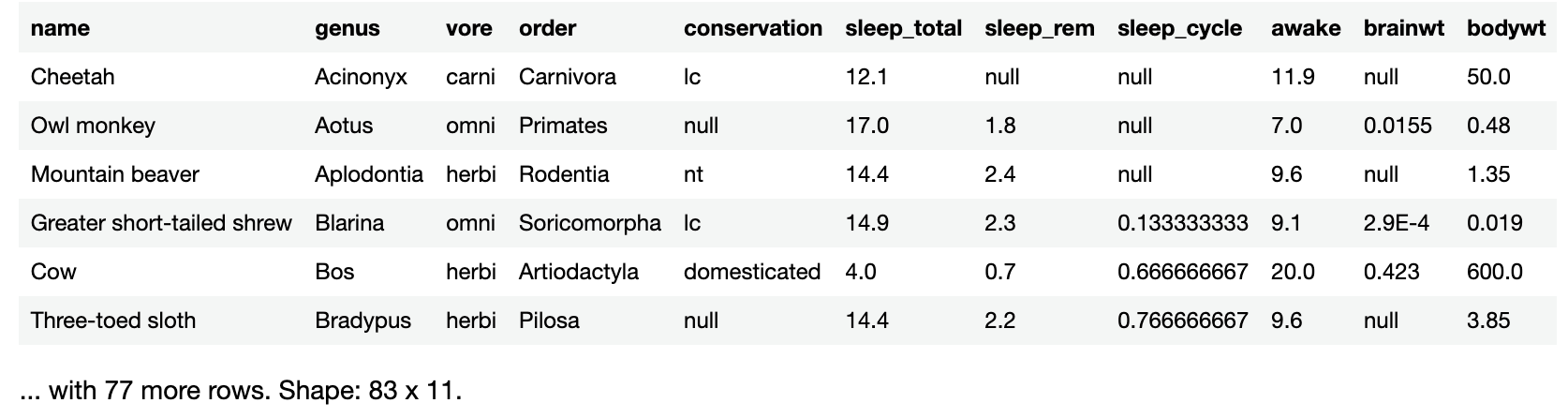
Notice that krangl tells you how many more rows there are in the data frame, 77 in this case, as well as the data frame’s dimensions: 83 rows and 11 columns. This is important because it tells you that while krangl is only showing you the first 6 rows, sleepData actually has 83 rows of data.

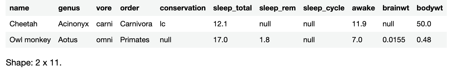
To see only the first n rows of the data frame, you can use the head() method. Run the following in a new code cell:

sleepData.head()

The notebook will respond by returning a data frame made up of the first five rows of sleepData:

head() returns a new data frame made from the first n rows of the original data frame. By default, n is 5.

Try getting the first 20 rows of sleepData by running the following in a new code cell:

sleepData.head(20)

You’ll see these results:

The result is a data frame consisting of the first 20 rows of sleepData, with the first six rows displayed onscreen. The text at the bottom of the data frame shows you how many rows you’re not seeing, as well as the data frame’s dimensions.

head() has a counterpart, tail(), which returns a new data frame made up of the last n rows of the original data frame. As with head(), the default value for n is 5.

Run the following in a new code cell:

val lastFew = sleepData.tail()
lastFew

The notebook will respond by creating and displaying lastFew, a data frame that contains the last 5 rows of sleepData:

Extracting a slice() from the Data Frame

Suppose you weren’t interested in the first or last n rows of the data frame, but a section in the middle. That’s where the slice() method comes in. Given an integer range, it creates a new data frame consisting of the rows specified in the range.

Run the following in a new code cell:

val selection = sleepData.slice(30..34)
selection

This creates a new data frame, selection, and then displays its contents:

If you looked at the row for “Human” and thought, “Who actually gets eight hours of sleep?!” keep in mind that these numbers are averages.

Learning that slice() Indexes Start at 1, not 0

Krangl borrows the DataFrame‘s slice()method from the dplyr library.

Dplyr is a library for R, where the first index of a collection type is 1. This is known as one-based array indexing.

In Kotlin, and most other programming languages, the first index of a collection type is 0.

krangl makes it easy for R programmers to make the leap to doing Kotlin sdata science. One of the ways to meet this goal would be to make krangl’s version of slice() work exactly like dplyr’s, right down to using 1 as the index for the first row in the data frame.

It’s time to do a little exploring.

Exploring the Data

Look back at the code cell where you used head() to see the first 5 rows of sleepData:

The first animal in the list is the cheetah. Try using DataFrame’s rows property and rows elementAt() method to retrieve the row whose index is 0:

sleepData.rows.elementAt(0)

You should see this result:

{name=Cheetah, genus=Acinonyx, vore=carni, order=Carnivora, conservation=lc, sleep_total=12.1, sleep_rem=null, sleep_cycle=null, awake=11.9, brainwt=null, bodywt=50.0}

This makes sense as rows is a Kotlin Iterable and elementAt() is a method of Iterable. It makes sense that sleepData.rows.elementAt(0) would return an object representing the first row of sleepData.

Now, try approximating the same thing with slice(). The result will be of a different type: sleepData.rows.elementAt() returns a DataFrameRow, while slice() returns a whole DataFrame.

Run the following in a new code cell:

sleepData.slice(0..0)

The result will be an empty data frame; 11 columns, but no rows:

Now, try something else. Run the following in a new code cell:

sleepData.slice(1..1)

This time, you get a data frame with a single row; note the dimensions:

Try one more thing; run the following in a new code cell:

sleepData.slice(1..2)

This results in a data frame with two rows:

From these little bits of code, you can deduce that slice(a..b) returns a data frame that:

1. Starts with and includes row a from the original data frame.
2. Ends with and includes row b from the original data frame.
3. Counts rows starting from 1 rather than starting from 0.

Sorting Data

One of the simplest and most effective ways to make sense of a dataset is to sort it. Sorting data by one or more criteria makes it easier to see progressions and trends, determine the minimums and maximums for specific variables in your observations and spot outliers.

DataFrame’s sortedBy() method takes one or more column names as its arguments and returns a new data frame whose contents are sorted by the specified columns in the given order.

With sleepData, it would be beneficial to have a data frame where the animals are sorted by the number of hours they sleep each day, from least to most. The sleep_total column contains those values.

Enter the following into a new code cell:

sleepData.sortedBy("sleep_total")

You’ll see these results:

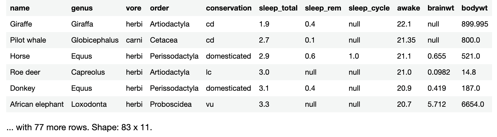
Sorting by hours of sleep per day makes it easy to see that the giraffe, an easily-spotted animal living among many predators, gets the least sleep.

Look a little farther down the data frame. Display rows 10 through 15 by running the following in a new code cell:

sleepData.sortedBy("sleep_total").slice(10..15)

Note that you’re using method chaining in the code above to produce a sorted data frame, and then get a smaller data frame made up of rows 10 through 15.

This is what you’ll see:

If you look at the rows for Goat and Tree hyrax, you’ll see that they both sleep 5.3 hours a day. The bodywt column, which shows body weight, also shows that goats are considerably larger than tree hyraxes, but the goat is first in the list.

Look a little further down the data frame with this code:

sleepData.sortedBy("sleep_total").slice(16..20)

This will display the next few rows:

The same situation with the goat and tree hyrax happens in the Gray hyrax and Genet rows. Both sleep for the same amount of time, and the heavier animal first in the list.

To deliberately sort the animals first by sleep time and then by body weight, you provide the names of those columns in that order. Run the following in a new code cell:

sleepData.sortedBy("sleep_total", "bodywt")

This time, the resulting table shows the animals sorted by the number of hours they sleep each day, from least to most. Where any animals sleep the same amount of time, the list will show them from lightest to heaviest.

sortedBy() has a counterpart, sortedByDescending(), which takes one or more column names as its arguments and returns a new data frame whose contents are sorted by the specified columns in the given order in descending order.

To see the animals listed in order from those who sleep the most to sleep the least, run the following in a new code cell:

sleepData.sortedByDescending("sleep_total")

The first two rows should show that of the 83 species in the dataset, brown bats sleep the most…almost 20 hours a day. I bet you wish you were a brown bat right now!

Filtering

Another key data operation is picking out only those observations whose variables meet specific criteria. This lets you focus on a section of the dataset or perhaps rule out outliers or other data you want to disqualify.

DataFrame provides the filter() method, which lets you specify columns and criteria for the columns’ values. Using these columns and criteria filter() creates a new data frame containing only rows whose column values meet the given criteria.

Filtering is a little easier to explain by example rather than describing it.

Learning the Basics of Filtering

Try creating new datasets based on animals in sleepData that meet certain criteria.

Suppose you want to look at the data for herbivores — animals that eat only plants. You can tell the type of food each animal eats by looking at the vore column. If you look at the first three animals in the list by running sleepData.head(3), you’ll see that the cheetah is a carnivore, the owl monkey is an omnivore, and the mountain beaver is a herbivore.

Create a herbivore-only data frame by running this code in a new code cell:

val herbivores = sleepData.filter { it["vore"] isEqualTo "herbi" }
println("This dataset has ${herbivores.nrow} herbivores.")
herbivores

You’ll see the following output:

This dataset has 32 herbivores.

Both the println() function and the metadata below the table inform you that the new data frame, herbivores, has 32 rows. That’s considerably fewer rows than sleepData, which contains 83.

filter() takes a single argument: A lambda that acts as the criteria for which rows should go into the new data frame. Let’s take a closer look at that lambda:

• When a lambda has a single parameter, you can reference that parameter using the implicit built-in name; it. In this case, it contains a reference to the sleepData data frame.
• Since it refers to sleepData, it["vore"] is a reference to a DataCol instance — a data frame column. In this case, it’s the vore column.
• isEqualTo is a method of DataCol. Given a column and a comparison value, it returns a BooleanArray with as many elements as the column has rows. For each row in the column, the element contains true if the value in the row matches the comparison value; otherwise it contains false. Note that isEqualTo is an infix function, which allows you to call it using the syntax it["vore"] isEqualTo "herbi" instead of using the standard syntax of it["vore"].isEqualTo("herbi"). The infix syntax feels more like natural language, but you can also use the standard syntax if you prefer.
• filter() uses the BooleanArray produced by the lambda to determine which rows from the original data frame go into the resulting data frame. A row that has a corresponding true element in the BooleanArray will appear in the resulting data frame.

It’s time to do a little more filtering.

Suppose you want to create a new dataset consisting of only the herbivores with a bodyweight of 200 kilograms (441 pounds) or more. Do this by running the following in a new code cell:

val heavyHerbivores = herbivores.filter { it["bodywt"] ge 200 }
heavyHerbivores

Note that this time, the comparison function in the lambda is ge, which is short for “greater than or equal to”. Here’s a quick list of the numeric comparison functions that you can use in a filter() lambda and when to use them:

• eq or isEqualTo: When you want to create a filter so that the resulting dataset contains only rows where the data in the given column is equal to the given value.
• ge: When you want to create a filter so that the resulting dataset contains only rows where the data in the given column is greater than or equal to the given value.
• gt: When you want to create a filter so that the resulting dataset contains only rows where the data in the given column is greater than the given value.
• le: When you want to create a filter so that the resulting dataset contains only rows where the data in the given column is less than or equal to the given value.
• lt: When you want to create a filter so that the resulting dataset contains only rows where the data in the given column is less than the given value.

The resulting data frame, heavyHerbivores, contains only 6 rows:

If you look at the sleep_total column, you’ll see that the best-rested of the bunch is the Brazilian tapir, which gets just over 4 hours of sleep a day. It seems that larger herbivores don’t sleep much, probably because they’re prime targets for predators. This is the kind of insight that you can get from judicious filtering.

Filtering With Negation

Imagine you wanted a data frame containing the animals that aren’t herbivores? You may have noticed that there isn’t a notEqualTo or ne in the list of comparison functions.

krangl’s approach for cases like this is to extend BooleanArray to give it a not() method. When called, this method negates every element in the array: true values become false, and false values become true.

Enter the following in a new code cell to see how you can use not() to create a data frame of all the non-herbivores:

val nonHerbivores = sleepData.filter { (it["vore"] eq "herbi").not() }
nonHerbivores

This works because it["vore"] eq "herbi" creates a BooleanArray specifying which rows contain herbivores. Calling not() on that array inverts its contents, making it a BooleanArray specifying which rows do not contain herbivores.

The output shows some carnivores, insectivores, omnivores, and one animal for which the vore value was not provided, the vesper mouse.

Filtering With Multiple Criteria

In addition to not(), krangl extends BooleanArray with the AND and OR infix functions. Using AND, you could have created and displayed a dataset of heavy herbivores by running this code instead:

val alsoHeavyHerbivores = sleepData
 .filter { 
 (it["vore"] eq "herbi") AND 
 (it["bodywt"] gt 30) 
 }
alsoHeavyHerbivores

Fancier Text Filtering

In addition to seeing if the contents of a column are equal to, greater than or less than a given value, you can do some fancier text filtering with the help of DataCol’s isMatching() method.

This is another method that’s easier to demonstrate than explain, so run the following in a new code cell:

val monkeys = sleepData.filter { it["name"].isMatching<String> { contains("monkey") } }
monkeys

This will result in a data frame containing only those animals with “monkey” in their name. The lambda that you provide to isMatching() should accept a string argument and return a boolean. You’ll find functions such as startsWith(), endsWith(), contains() and matches() useful within that lambda.

Removing Columns

With filtering, you were removing rows from a data frame. You’ll often find that removing columns whose information isn’t needed at the moment is also useful. DataFrame has a couple of methods that you can use to create a new data frame from an existing one, but with fewer columns.

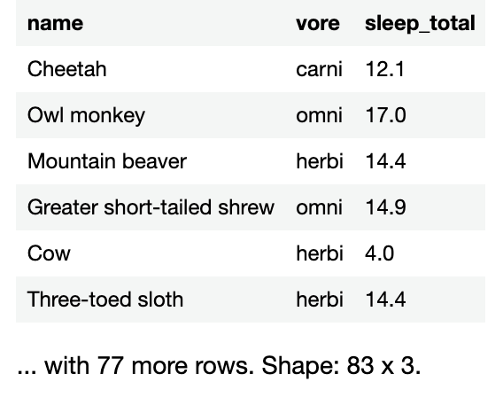
select() creates a new data frame from an existing one, but only with the columns whose names you specify.

Run the following code in a new cell to see select() in action:

val simplifiedSleepData = sleepData.select("name", "vore", "sleep_total", "sleep_rem")
simplifiedSleepData

You’ll see with a table that has only the columns whose names you specified: name, vore, sleep_total, and sleep_rem.

remove() creates a new data frame from an existing one, but without the columns whose names you specify.

Run the following code in a new cell to see remove() in action:

val evenSimplerSleepData = simplifiedSleepData.remove("sleep_rem")
evenSimplerSleepData

You’ll see this result:

Performing Complex Data Operations

So far, you’ve been working with operations that work with observations on an individual basis. While useful, the real power of data science comes from aggregating data — collecting many units of data into one.

Calculating Column Statistics

DataCol provides a number of handy math and statistics methods for often-performed calculations on numerical columns.

The simplest way to demonstrate how they work is to show you these functions in action on a given column, such as sleep_total.

Run the following code in a new code cell to see these functions in action:

val sleepCol = sleepData["sleep_total"]
println("The mean sleep period is ${sleepCol.mean(removeNA=true)} hours.")
println("The median sleep period is ${sleepCol.median(removeNA=true)} hours.")
println("The standard deviation for the sleep periods is ${sleepCol.sd(removeNA=true)} hours.")
println("The shortest sleep period is ${sleepCol.min(removeNA=true)} hours.")
println("The longest sleep period is ${sleepCol.max(removeNA=true)} hours.")

These methods take a boolean argument, removeNA, which specifies whether to exclude missing values from the calculation. The default value is false, but it’s generally better to set this value to true.

Grouping

In the previous exercise, you calculated the mean, median, and other statistical information about the entire set of animals in the dataset. While those results might be useful, you’re likely to get more insights by doing the same calculations on smaller sets of animals with something in common. Grouping allows you to create these smaller sets.

Given one or more column names, DataFrame’s group() method creates a new data frame from an existing one, but organized into a set of smaller data frames. called groups. Each group consists of rows that had the same values for the specified columns.

Don’t worry if the previous paragraph confused you. This is yet another one of those situations where showing is better than telling.

Break sleepData‘s animals into groups based on the food they eat. There should be a carnivore group, an omnivore group, a herbivore group, etc. The vore column specifies what an animal eats, so you’ll provide that column name to the group() method.

Run the following in a new code cell:

val groupedData = sleepData.groupBy("vore")

This creates a new data frame named groupedData.

If you try to display groupedData‘s contents by entering its name into a new code cell and running it, the output will be confusing:

Grouped by: *[vore]
A DataFrame: 5 x 11
 name genus vore order conservation sleep_total sleep_rem
1 Cheetah Acinonyx carni Carnivora lc 12.1 
2 Northern fur seal Callorhinus carni Carnivora vu 8.7 1.4
3 Dog Canis carni Carnivora domesticated 10.1 2.9
4 Long-nosed armadillo Dasypus carni Cingulata lc 17.4 3.1
5 Domestic cat Felis carni Carnivora domesticated 12.5 3.2
and 4 more variables: awake, brainwt, bodywt

The output says that the data frame is grouped by vore and has 5 rows and 11 columns. The problem is that the default way to display the contents of a data frame works only for ungrouped data frames. You have to do a little more work to display the contents of a grouped data frame.

Run and enter the following in a new code cell:

groupedData.groups()

groups() returns the list of the data frame’s groups, and remember, groups, are just data frames.

You’ll see 5 data frames in a row. Each of these data frames contains rows with a common value in their vore column. There’s one group for “carni”, one called “omni”, and so on.

DataFrame has a count() method that’s very useful for groups; it returns a data frame containing the count of rows for each group.

Run and enter the following in a new code cell:

groupedData.count()

This is the result:

Any data frame operation performed on a grouped data frame is done on a per-group basis.

For example, sorting a grouped data frame creates a new data frame with individually sorted groups. You can see this for yourself by running the following in a new code cell:

val sortedGroupedData = groupedData.sortedBy("name")
sortedGroupedData.groups()

Summarizing

Summarizing is the act of applying calculations to a grouped data frame on a per-group basis. Calculate sleep statistics for the grouped data frame.

Run the following code in a new code cell:

groupedData
 .summarize(
 "Mean daily total sleep (hours)" to { it["sleep_total"].mean(removeNA=true) },
 "Mean daily REM sleep (hours)" to { it["sleep_rem"].mean(removeNA=true) }
 )

The output, as the summarize() method name suggests, is a nice summary:

Now, improve on the summary by sorting it.

Run the following in a new code cell:

groupedData
 .summarize(
 "Mean daily total sleep (hours)" to { it["sleep_total"].mean(removeNA=true) },
 "Mean daily REM sleep (hours)" to { it["sleep_rem"].mean(removeNA=true) }
 )
 .sortedBy("Mean daily total sleep (hours)")

Now the summary lists the groups sorted by how much sleep they get, from least to most:

From this summary, you’ll see that herbivores sleep the least, carnivores and omnivores get a little more sleep, and insectivores get the most sleep, spending more time asleep than awake.

The summary might lead you to a set of hypotheses that you might want to test with more experiments. One of the more obvious ones is that herbivores are what carnivores and omnivores eat, which means that they have to stay alert and sleep less.

In data science, you’ll find that an often-used workflow is one that consists of doing the following to a data frame in this order:

• Filtering / Selecting
• Grouping
• Summarizing
• Sorting

Importing Data

While you can load data into a data frame using code, it’s quite unlikely that you’ll be doing it that way. In most cases, you’ll work with data saved in a commonly-used file format.

Data entry is a big and often overlooked part of data science, and spreadsheets remain the preferred data entry tool, even after all these years. They make it easy to enter tables of data, and they’ve been around long enough for them to become a tool that even casual computer users understand.

While spreadsheet applications save their files in a proprietary format, they can also export their data in a couple of standard plain-text formats that other applications can easily read: .csv and .tsv.

Reading .csv Data

One of the most common file formats for data is .csv, which is short for comma-separated value.

Each line in a .csv file represents a row of data, and within each line, each column value is delineated by commas. The first row contains column titles by default, while the remaining rows contain the data.

For example, here’s how the data frame you created earlier would be represented in .csv form:

language,developer,year_first_appeared,preferred
Kotlin,JetBrains,2011,true
Java,James Gosling,1995,false
Swift,Chris Lattner et al.,2014,true
Objective-C,Tom Love and Brad Cox,1984,false
Dart,Lars Bak and Kasper Lund,2011,true

Given a URL for a remote file, the readCSV() method of the DataFrame class reads .csv data and uses it to create a new data frame.

Enter and run the following in a new code cell:

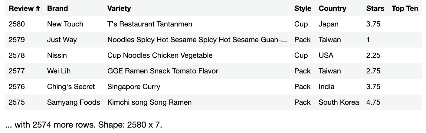
val ramenRatings = DataFrame.readCSV("https://koenig-media.raywenderlich.com/uploads/2021/07/ramen-ratings.csv")
ramenRatings

You’ll see the following result:

You could’ve just as easily downloaded the file and read it locally using readCSV(), as it’s versatile enough to work with both URLs and local filepaths.

Reading .tsv Data

The .csv format has one major limitation; since it uses commas as a data separator, the data can’t contain commas. This rules out certain kinds of data, especially text data containing full sentences.

This is where the .tsv format is useful. Rather than delimiting data with commas, the .tsv format uses tab characters, which are control characters that aren’t typically part of text created by humans.

The DataFrame class’ readTSV() method works like readCSV(), except that it initializes a data frame with the data from a .tsv file.

Run this code in a new code cell:

val restaurantReviews = DataFrame.readTSV("https://koenig-media.raywenderlich.com/uploads/2021/07/restaurant-reviews.tsv")
restaurantReviews

It should produce the following output:

You can see that any written text can appear.

Where to Go From Here?

You can download the Jupyter Notebook files containing all the code from the exercises above by clicking on the Download Materials button at the top or bottom of the tutorial.

You’ve completed your first steps in data science with Kotlin. The data frame basics covered here are the basis of many Jupyter Notebook projects, and they’re just the beginning.

There’s a lot more ground you can cover while exploring Kotlin-powered data science. Here are a few good starting points:

• Roman Belov’s presentation at KotlinConf 2019, Using Kotlin for Data Science. This is a grand tour of what you can do with Jupyter Notebook and the Kotlin Kernel, which includes drawing graphs as well as other libraries such as Kotlin NumPy and Apache Spark, and even using other “notebook” technologies like Apache Zeppelin.
• Kotlin Data Science Resources. A collection of showcase applications, Kotlin and Java libraries, resources for Kotlin and Python data science developers and other useful resources for your learning journey.
• Kotlin Jupyter Kernel for Data Analysis: Reviewing NFL Win Probability Models. If you’re looking an example of Kotlin being used in a data science project, this March 2021 presentation for the San Diego Kotlin User Group is a good one. This project attempts to predict NFL teams’ odds of winning based on historical data.
• Data Science on the JVM with Kotlin and Zeppelin. This 2021 presentation for the Chicago Kotlin User Group shows Kotlin being used on a different “notebook” platform: Apache Zeppelin. Many of the ideas shown in this video can be applied to Jupyter Notebook projects.

We hope you enjoyed this tutorial. If you have any questions or comments, please join the forum discussion below!