Prediction Intervals for Random Forests

I previously knew about generating prediction intervals via random forests by calculating the quantiles over the forest. (See this prior python post of mine for getting the individual trees). A recent set of answers on StackExchange show a different approach – apparently the individual tree approach tends to be too conservative (coverage rates higher than you would expect). Those Cross Validated posts have R code, figured it would be good to illustrate in python code how to generate these prediction intervals using random forests.

So first what is a prediction interval? I imagine folks are more familiar with confidence intervals, say we have a regression equation y = B1*x + e, you often generate a confidence interval around B1. Imagine we use that equation to make a prediction though, y_hat = B1*(x=10), here prediction intervals are errors around y_hat, the predicted value. They are actually easier to interpret than confidence intervals, you expect the prediction interval to cover the observations a set percentage of the time (whereas for confidence intervals you have to define some hypothetical population of multiple measures).

Prediction intervals are often of more interest for predictive modeling, say I am predicting future home sale value for flipping houses. I may want to generate prediction intervals that cover the value 90% of the time, and only base my decisions to buy based on the much lower value (if you are more risk averse). Imagine I give you the choice of buy a home valuated at 150k - 300k after flipped vs a home valuated at 230k-250k, the upside for the first is higher, but it is more risky.

In short, this approach to generate prediction intervals from random forests relies on out of bag error metrics (it is sort of like a for free hold out sample based on the bootstrapping approach random forest uses). And based on the residual distribution, one can generate forecast intervals (very similar to Duan’s smearing).

To illustrate, I will use a dataset of emergency room visits and time it took to see a MD/RN/PA, the NHAMCS data. I have code to follow along here, but I will walk through it in this post (that code has some nice functions for data definitions for the NHAMCS data).

At work I am working on a project related to unnecessary emergency room visits, and I actually went to the emergency room in December (for a Kidney stone). So I am interested here in generating prediction intervals for the typical time it takes to be served in an ER to see if my visit was normal or outlying.

Example Python Code

First for some set up, I import the libraries I am using, and read in the emergency room use data:

import numpy as np
import pandas as pd
from nhanes_vardef import * #variable definitions
from sklearn.ensemble import RandomForestRegressor
from sklearn.model_selection import train_test_split

# Reading in fixed width data
# Can download this data from 
# https://ftp.cdc.gov/pub/Health_Statistics/NCHS/Datasets/NHAMCS/
nh2019 = pd.read_fwf('ED2019',colspecs=csp,header=None)
nh2019.columns = list(fw.keys())

Here I am only going to work with a small set of the potential variables. Much of the information wouldn’t make sense to use as predictors of time to first being seen (such as subsequent tests run). One thing I was curious about though was if I changed my pain scale estimate would I have been seen sooner!

# WAITTIME
# PAINSCALE [- missing]
# VDAYR [Day of Week]
# VMONTH [Month of Visit]
# ARRTIME [Arrival time of day]
# AGE [top coded at 95]
# SEX [1 female, 2 male]
# IMMEDR [triage]
#  9 = Blank
#  -8 = Unknown
#  0 = ‘No triage’ reported for this visit but ESA does conduct nursing triage
#  1 = Immediate
#  2 = Emergent
#  3 = Urgent
#  4 = Semi-urgent
#  5 = Nonurgent
#  7 = Visit occurred in ESA that does not conduct nursing triage 

keep_vars = ['WAITTIME','PAINSCALE','VDAYR','VMONTH','ARRTIME',
             'AGE','SEX','IMMEDR']
nh2019 = nh2019[keep_vars].copy()

Many of the variables encode negative values as missing data, so here I throw out visits with a missing waittime. I am lazy though and the rest I keep as is, with enough data random forests should sort out all the non-linear effects no matter how you encode the data. I then create a test split to evaluate the coverage of my prediction intervals out of sample for 2k test samples (over 13k training samples).

# Only keep wait times that are positive
mw = nh2019['WAITTIME'] >= 0
print(nh2019.shape[0] - mw.sum()) #total number missing
nh2019 = nh2019[mw].copy()

# Test hold out sample to show
# If coverage is correct
train, test = train_test_split(nh2019, test_size=2000, random_state=10)
x = keep_vars[1:]
y = keep_vars[0]

Now we can fit our random forest model, telling python to keep the out of bag estimates.

# Fitting the model on training data
regr = RandomForestRegressor(n_estimators=1000,max_depth=7,
  random_state=10,oob_score=True,min_samples_leaf=50)
regr.fit(train[x], train[y])

Now we can use these out of bag estimates to generate error intervals around our predictions based on the test oob error distribution. Here I generate 50% prediction intervals.

# Generating the error distribution
resid = train[y] - regr.oob_prediction_
# 50% interval
lowq = resid.quantile(0.25)
higq = resid.quantile(0.75)
print((lowq,higq)) 
# negative much larger
# so tends to overpredict time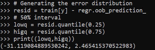

Even 50% here are quite wide (which could be a function of both the data has a wide variance as well as the model is not very good). But we can test whether our prediction intervals are working correctly by seeing the coverage on the out of sample test data:

# Generating predictions on out of sample data
test_y = regr.predict(test[x])
lowt = (test_y + lowq).clip(0) #cant have negative numbers
higt = (test_y + higq)

cover = (test[y] >= lowt) & (test[y] <= higt)
print(cover.mean())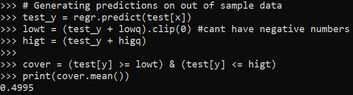

Pretty much spot on. So lets see what the model predicts my referent 50% prediction interval would be (I code myself a 2 on the IMMEDR scale, as I was billed a CPT code 99284, which those should line up pretty well I would think):

# Seeing what my referent time would be
myt = np.array([[6,4,12,930,36,2,6]])
mp = regr.predict(myt)
print(mp)
print( (mp+lowq).clip(0), (mp+higq) )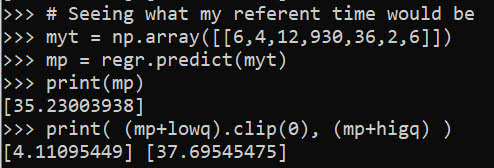

So a predicted mean of 35 minutes, and a prediction interval of 4 to 38 minutes. (These intervals based on the residual quantiles are basically non-parametric, and don’t have any strong assumptions about the distribution of the underlying data.)

To first see the triage nurse it probably took me around 30 minutes, but to actually be treated it was several hours long. (I don’t think you can do that breakdown in this dataset though.)

We can do wider intervals, here is a screenshot for 80% intervals:

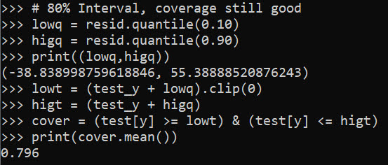
You can see that they are quite wide, so probably not very effective in identifying outlying cases. It is possible to make them thinner with a better model, but it may just be the variance is quite wide. For folks monitoring time it takes for things (whether time to respond to calls for service for police, or here be served in the ER), it probably makes sense to build models focusing on quantiles, e.g. look at median time served instead of mean.