

What Is the Frank Matrix?
source link: https://nhigham.com/2022/01/25/what-is-the-frank-matrix/
Go to the source link to view the article. You can view the picture content, updated content and better typesetting reading experience. If the link is broken, please click the button below to view the snapshot at that time.
What Is the Frank Matrix?
The 
![\notag F_n = \left[\begin{array}{*{6}c} n & n-1 & n-2 & \dots & 2 & 1 \\ n-1 & n-1 & n-2 & \dots & 2 & 1 \\ 0 & n-2 & n-2 & \dots & 2 & 1 \\[-3pt] \vdots & 0 & \ddots & \ddots & \vdots & 1 \\[-3pt] \vdots & \vdots & \dots & 2 & 2 & 1 \\ 0 & 0 & \dots & 0 & 1 & 1 \\ \end{array}\right]](https://s0.wp.com/latex.php?latex=%5Cnotag+++F_n+%3D+++%5Cleft%5B%5Cbegin%7Barray%7D%7B%2A%7B6%7Dc%7D+++n++++++%26+n-1++++%26+n-2++++%26+%5Cdots++%26+2++++++%26+1+%5C%5C+++n-1++++%26+n-1++++%26+n-2++++%26+%5Cdots++%26+2++++++%26+1+%5C%5C+++0++++++%26+n-2++++%26+n-2++++%26+%5Cdots++%26+2++++++%26+1+%5C%5C%5B-3pt%5D+++%5Cvdots+%26+0++++++%26+%5Cddots+%26+%5Cddots+%26+%5Cvdots+%26+1+%5C%5C%5B-3pt%5D+++%5Cvdots+%26+%5Cvdots+%26+%5Cdots++%26+++2++++%26+2++++++%26+1+%5C%5C+++0++++++%26+0++++++%26+%5Cdots++%26+++0++++%26+1++++++%26+1+%5C%5C+++%5Cend%7Barray%7D%5Cright%5D+&bg=ffffff&fg=222222&s=0&c=20201002)
was introduced by Frank in 1958 as a test matrix for eigensolvers.
Determinant
Taking the Laplace expansion about the first column, we obtain 


In MATLAB, the computed determinant of the matrix and its transpose can be far from the exact values of 
>> n = 20; F = anymatrix('gallery/frank',n);
>> [det(F), det(F')]
ans =
   1.0000e+00  -1.4320e+01
>> n = 49; F = anymatrix('gallery/frank',n); det(F)
ans =
    -1.406934439401568e+45
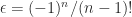
This behavior illustrates the sensitivity of the determinant rather than numerical instability in the evaluation and it is very dependent on the arithmetic (different results may be obtained in different releases of MATLAB). The sensitivity can be seen by noting that

which means that changing the 


Inverse and Condition Number
It is easily verified that
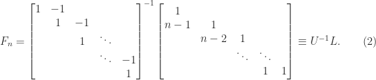
Hence 
From (1) we see that 
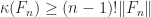
for any subordinate matrix norm, showing that the condition number grows very rapidly with 


Eigenvalues
Denote by 


Using (3), one can show by induction that
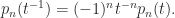
This means that the eigenvalues of 

>> charpoly( anymatrix('gallery/frank',6) )
ans =
     1   -21   120  -215   120   -21     1
>> charpoly( anymatrix('gallery/frank',7) )
ans =
     1   -28   231  -665   665  -231    28    -1
Since 

If each eigenvalue of an 


>> n = 9; F = anymatrix('gallery/frank',n);
>> [V,D,cond_evals] = condeig(F); evals = diag(D);
>> [~,k] = sort(evals,'descend');
>> [evals(k) cond_evals(k)]
ans =
   2.2320e+01   1.9916e+00
   1.2193e+01   2.3903e+00
   6.1507e+00   1.5268e+00
   2.6729e+00   3.6210e+00
   1.0000e+00   6.8615e+01
   3.7412e-01   1.5996e+03
   1.6258e-01   1.1907e+04
   8.2016e-02   2.5134e+04
   4.4803e-02   1.4762e+04
Notes
Frank found that
References
This is a minimal set of references, which contain further useful references within.
- Werner Frank, Computing Eigenvalues of Complex Matrices by Determinant Evaluation and by Methods of Danilewski and Wielandt, J. Soc. Indust. Appl. Math. 6(4), 378–392, 1958.
- Efruz Özlem Mersin and Mustafa Bahçsi, Sturm Theorem for the Generalized Frank Matrix, Hacettepe Journal of Mathematics and Statistics 50, 1002–1011, 2021.
- J. H. Wilkinson, Error Analysis of Floating-Point Computation, Numer. Math. 2(1), 319–340, 1960.
- J. H. Wilkinson, The Algebraic Eigenvalue Problem, Oxford University Press, 1965, Section 5.45.
Posted on January 25, 2022January 25, 2022 by Nick HighamPosted in what-is
Post navigation
One thought on “What Is the Frank Matrix?”
-
Some time ago, I had devised a modified version of the Frank matrix, using the ideas in Varah’s paper (https://doi.org/10.1137/0907056). In particular, using his recipe with the Clement-Kac matrix (MATLAB’s gallery(‘clement’)), the $n\times n$ upper Hessenberg matrix with entries $h_{i,j} = j (n-j)+[i \leq j]$ (where $[p]$ is an Iverson bracket) has determinant $1$ and eigenvalues $\left(\frac{k}{2}+\sqrt{1+\frac{k^2}{4}}\right)^2$, $k=-(n-1), -(n-3), \dots, n-1$. It seems to be even more badly behaved than the original.

Leave a Reply Cancel reply
Recommend
About Joyk
Aggregate valuable and interesting links.
Joyk means Joy of geeK