

Using SingleStore as a Geospatial Database
source link: https://dzone.com/articles/using-singlestore-as-a-geospatial-database
Go to the source link to view the article. You can view the picture content, updated content and better typesetting reading experience. If the link is broken, please click the button below to view the snapshot at that time.

Abstract
SingleStore is a multi-model database system. In addition to relational data, it supports key-value, JSON, full-text search, geospatial, and time series. A previous article showed SingleStore's ability to manage Time Series data.
In this article, we'll explore geospatial data. We'll use data for the London boroughs and data for the London Underground. We'll use these datasets to perform a series of geospatial queries to test SingleStore's ability to work with geospatial data. We'll also discuss an extended example using the London Underground data for a practical use case: finding the shortest path between two points in a network. Finally, we'll create London Underground visualizations using Folium and Streamlit.
The SQL scripts, Python code, and notebook files used in this article are available on GitHub. The notebook files are available in DBC, HTML, and iPython formats.
Introduction
In the previous article (mentioned above), we noted the problems of using Polyglot Persistence for managing diverse data and processing requirements. We also discussed how SingleStore would be an excellent solution for time series data, providing business and technical benefits. This article will focus on geospatial data and how SingleStore can offer a unified approach to storing and querying alphanumeric and geospatial data.
To begin with, we need to create a free Managed Service account on the SingleStore website, and a free Community Edition (CE) account on the Databricks website. At the time of writing, the Managed Service account from SingleStore comes with $500 of credits. This is more than adequate for the case study described in this article. For Databricks CE, we need to sign-up for the free account rather than the trial version. We are using Spark because, as noted in a previous article, Spark is great for ETL with SingleStore.
The data for London boroughs can be downloaded from the London Datastore. The file we will use is statistical-gis-boundaries-london.zip. This file is 27.34 MB in size. We will need to perform some transformations on the data provided to use the data with SingleStore. We will discuss these transformations shortly.
The data for the London Underground can be obtained from Wikimedia. It is available in CSV format as stations, routes, and line definitions. This dataset appears to be widely used but lags behind the latest developments on the London Underground. However, it is sufficient for our needs and could be easily updated in the future.
A version of the London Underground dataset can also be found on GitHub, with the extra column time added to routes. This will help find the shortest path, which we will discuss later.
An updated set of the London Underground CSV files can be downloaded from the GitHub page for this article.
To summarize:
- Download the zip file from the London Datastore.
- Download the three London Underground CSV files from the GitHub page for this article.
Configure Databricks CE
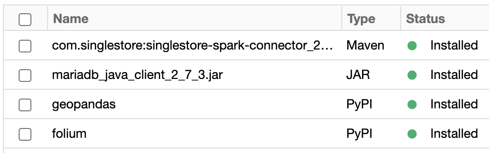
This previous article provides detailed instructions on how to configure Databricks CE for use with SingleStore. We can use those exact instructions for this use case. As shown in Figure 1, in addition to the SingleStore Spark Connector and the MariaDB Java Client jar file, we need to add GeoPandas and Folium. These can be added using PyPI.
Upload CSV Files
To use the three London Underground CSV files, we need to upload them into the Databricks CE environment. This previous article provides detailed instructions on how to upload a CSV file. We can use those exact instructions for this use case.
London Boroughs Data
Convert London Boroughs Data
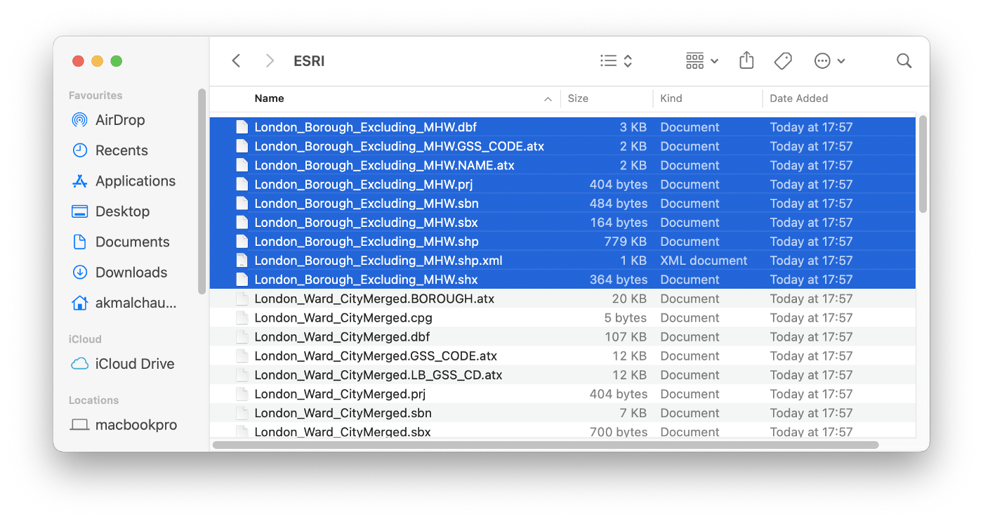
The zip file we downloaded needs to be unzipped. Inside, there will be two folders: ESRI and MapInfo. Inside the ESRI folder, we are interested in the files beginning with London_Borough_Excluding_MHW. There will be various file extensions, as shown in Figure 2.
We need to convert the data in these files to the well-known text (WKT) format for SingleStore. To do this, we can follow the advice on the SingleStore website for loading geospatial data into SingleStore.
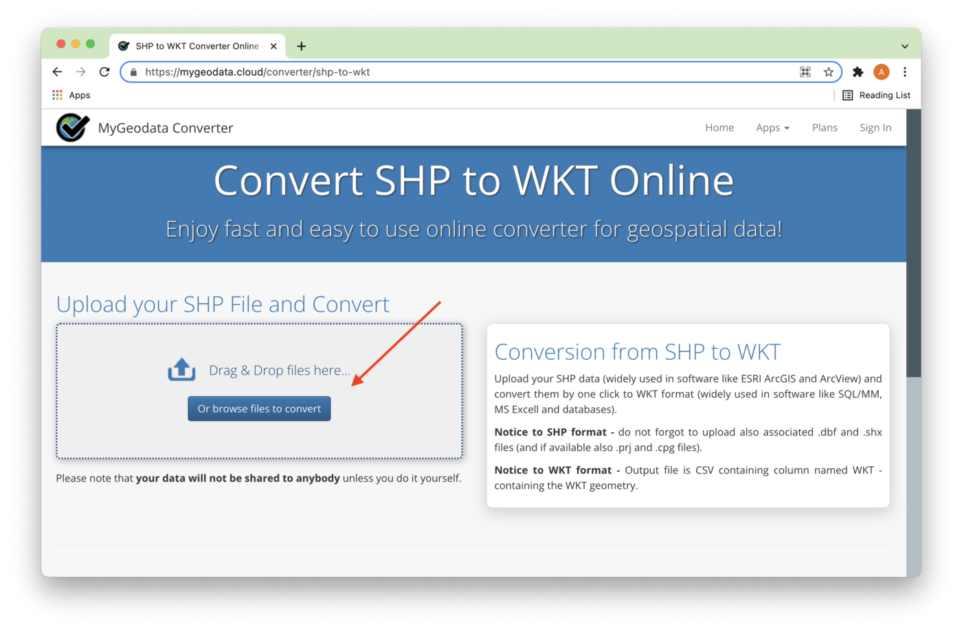
The first step is to use the MyGeodata Converter tool. We can drag and drop files or browse files to convert, as shown in Figure 3.
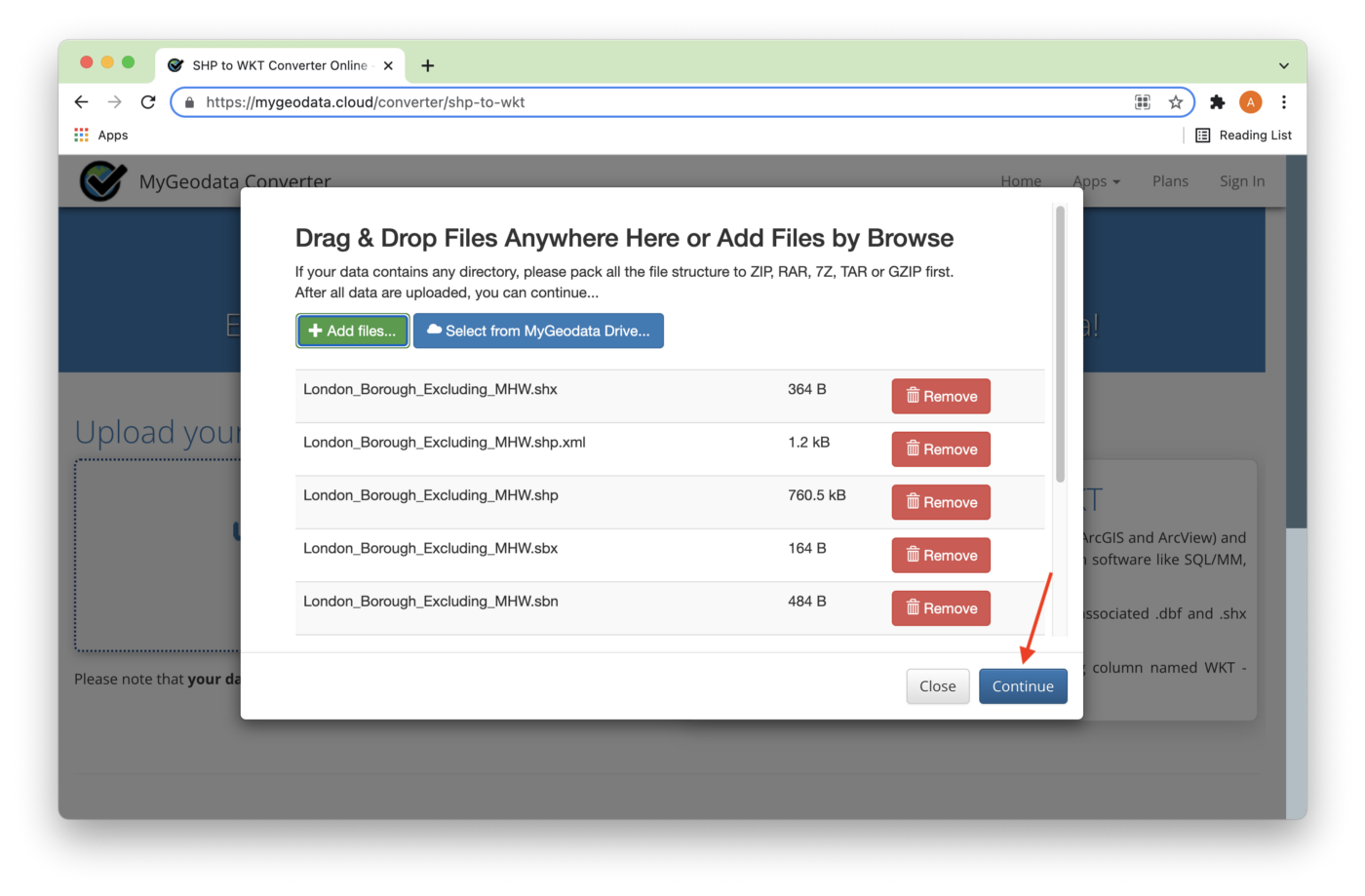
All nine files highlighted in Figure 2 have been added, as shown in Figure 4. Next, we'll click Continue.
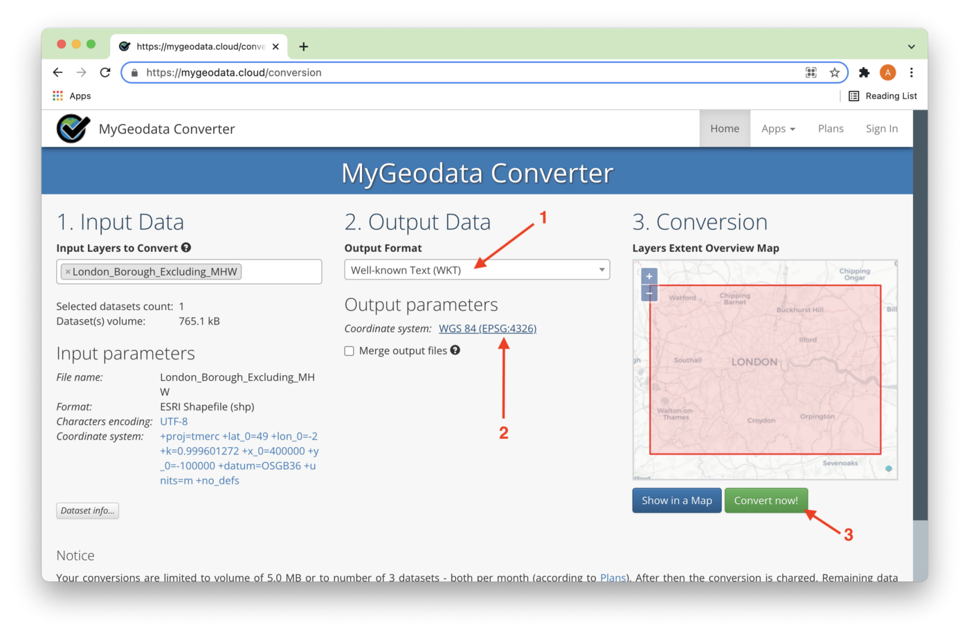
On the next page, we need to check that the output format is WKT, that the Coordinate system is WGS 84,and click convert now! as shown in Figure 5.
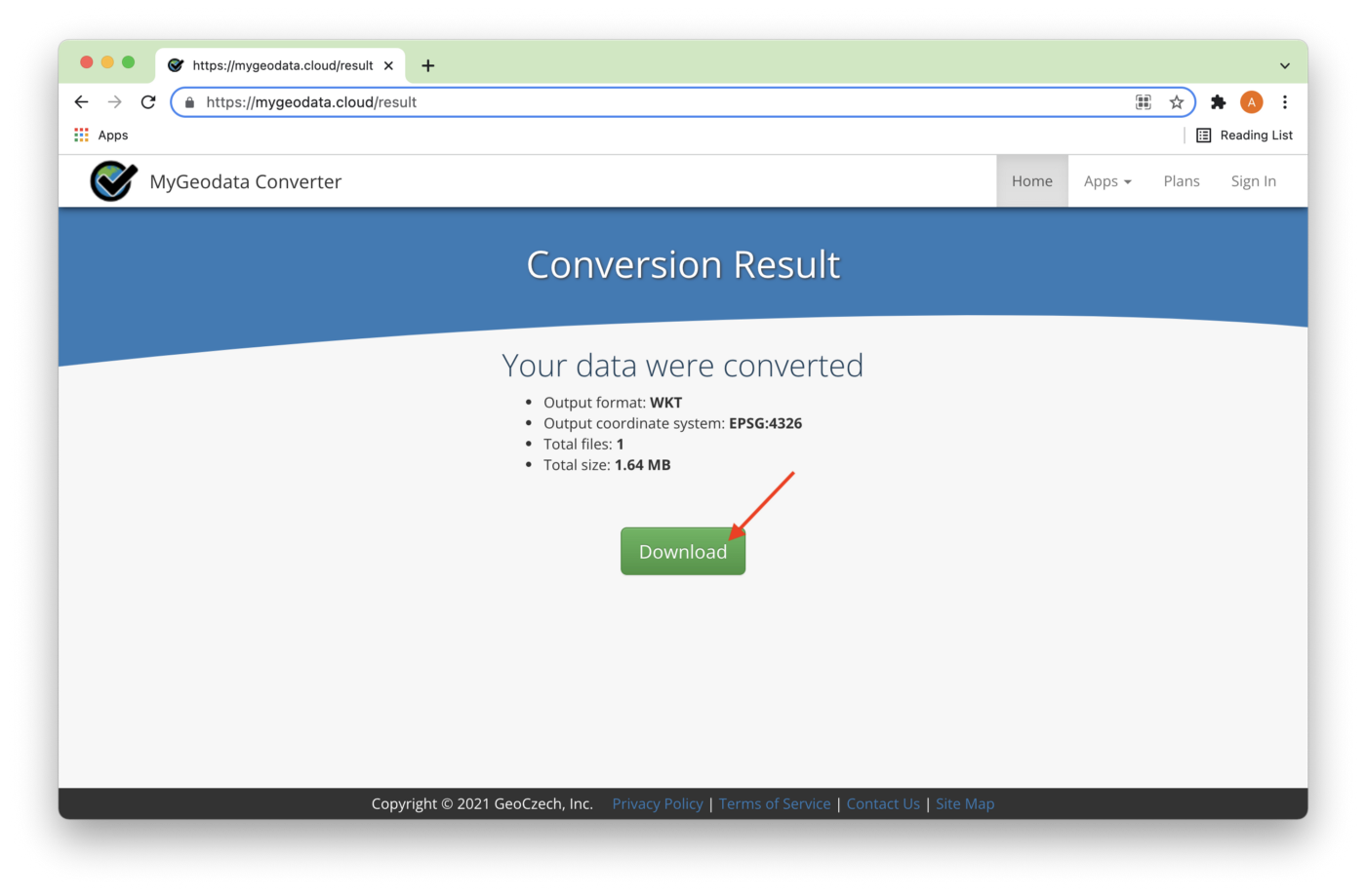
The conversion result can be downloaded, as shown in Figure 6.
This will download a zip file that contains a CSV file called London_Borough_Excluding_MHW.csv. This file contains a header row and 33 rows of data. One column will be called WKT and have 30 rows of POLYGON data, and there will be three rows of MULTIPOLYGON data. We need to convert the MULTIPOLYGON data to POLYGON data. We can do this very quickly using GeoPandas.
Next, we'll also upload this CSV file to Databricks CE.
Create the London Boroughs Database Table
In our SingleStore Managed Service account, let's use the SQL Editor to create a new database. Call this geo_db, as follows:
CREATE DATABASE IF NOT EXISTS geo_db;
We'll also create a table, as follows:
USE geo_db;
CREATE ROWSTORE TABLE IF NOT EXISTS london_boroughs (
name VARCHAR(32),
hectares FLOAT,
geometry GEOGRAPHY,
centroid GEOGRAPHYPOINT,
INDEX(geometry)
);
SingleStore can store three main geospatial types: polygons, paths, and points. In the above table, GEOGRAPHY can hold polygon and path data. GEOGRAPHYPOINT can hold point data. In our example, the geometry column will contain the shape of each London borough and centroid will contain the approximate central point of each borough. As shown above, we can store this geospatial data alongside other data types, such as VARCHAR and FLOAT.
Data Loader for London Boroughs
Let's now create a new Databricks CE Python notebook. We'll call it Data Loader for London Boroughs. We'll attach our new notebook to our Spark cluster.
In a new code cell, let's add the following code to import several libraries:
import pandas as pd
import geopandas as gpd
from pyspark.sql.types import *
from shapely import wkt
Next, we'll define our schema:
geo_schema = StructType([
StructField("geometry", StringType(), True), StructField("name", StringType(), True), StructField("gss_code", StringType(), True), StructField("hectares", DoubleType(), True), StructField("nonld_area", DoubleType(), True), StructField("ons_inner", StringType(), True), StructField("sub_2009", StringType(), True), StructField("sub_2006", StringType(), True)])
Now we'll read our CSV using the schema we defined:
boroughs_df = spark.read.csv("/FileStore/London_Borough_Excluding_MHW.csv",header = True,
schema = geo_schema)
We'll drop some of the columns:
boroughs_df = boroughs_df.drop("gss_code", "nonld_area", "ons_inner", "sub_2009", "sub_2006")Let's now review the structure and contents of the data:
boroughs_df.show(33)
The output should be as follows:
+--------------------+--------------------+---------+
| geometry| name| hectares|
+--------------------+--------------------+---------+
|POLYGON ((-0.3306...|Kingston upon Thames| 3726.117|
|POLYGON ((-0.0640...| Croydon| 8649.441|
|POLYGON ((0.01213...| Bromley|15013.487|
|POLYGON ((-0.2445...| Hounslow| 5658.541|
|POLYGON ((-0.4118...| Ealing| 5554.428|
|POLYGON ((0.15869...| Havering|11445.735|
|POLYGON ((-0.4040...| Hillingdon|11570.063|
|POLYGON ((-0.4040...| Harrow| 5046.33|
|POLYGON ((-0.1965...| Brent| 4323.27|
|POLYGON ((-0.1998...| Barnet| 8674.837|
|POLYGON ((-0.1284...| Lambeth| 2724.94|
|POLYGON ((-0.1089...| Southwark| 2991.34|
|POLYGON ((-0.0324...| Lewisham| 3531.706|
|MULTIPOLYGON (((-...| Greenwich| 5044.19|
|POLYGON ((0.12021...| Bexley| 6428.649|
|POLYGON ((-0.1058...| Enfield| 8220.025|
|POLYGON ((0.01924...| Waltham Forest| 3880.793|
|POLYGON ((0.06936...| Redbridge| 5644.225|
|POLYGON ((-0.1565...| Sutton| 4384.698|
|POLYGON ((-0.3217...|Richmond upon Thames| 5876.111|
|POLYGON ((-0.1343...| Merton| 3762.466|
|POLYGON ((-0.2234...| Wandsworth| 3522.022|
|POLYGON ((-0.2445...|Hammersmith and F...| 1715.409|
|POLYGON ((-0.1838...|Kensington and Ch...| 1238.379|
|POLYGON ((-0.1500...| Westminster| 2203.005|
|POLYGON ((-0.1424...| Camden| 2178.932|
|POLYGON ((-0.0793...| Tower Hamlets| 2157.501|
|POLYGON ((-0.1383...| Islington| 1485.664|
|POLYGON ((-0.0976...| Hackney| 1904.902|
|POLYGON ((-0.0976...| Haringey| 2959.837|
|MULTIPOLYGON (((0...| Newham| 3857.806|
|MULTIPOLYGON (((0...|Barking and Dagenham| 3779.934|
|POLYGON ((-0.1115...| City of London| 314.942|
+--------------------+--------------------+---------+
We need to convert the rows with MULTIPOLYGON to POLYGON so, first, we'll create a Pandas DataFrame:
boroughs_pandas_df = boroughs_df.toPandas()
And then we'll convert the string to polygon for the geometry column using wkt.loads:
boroughs_pandas_df["geometry"] = boroughs_pandas_df["geometry"].apply(wkt.loads)
Now we'll convert to a GeoDataFrame:
boroughs_geo_df = gpd.GeoDataFrame(boroughs_pandas_df, geometry = "geometry")
This is so that we can use explode() to change the MULTIPOLYGON to POLYGON:
boroughs_geo_df = boroughs_geo_df.explode(column = "geometry", index_parts = False)
If we check the structure of the DataFrame:
boroughs_geo_df
We should not see any rows now with MULTIPOLYGON.
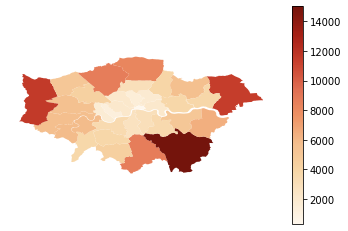
We can plot a map of the London boroughs, as follows:
map = boroughs_geo_df.plot(column = "hectares", cmap = "OrRd", legend = True)
map.set_axis_off()
This should render the image shown in Figure 7.
At this point, since a map is being rendered, the following needs to be added:
“Contains National Statistics data © Crown copyright and database right [2015]” and “Contains Ordnance Survey data © Crown copyright and database right [2015]”
We can also add a new column that contains the centroid for each borough:
boroughs_geo_df = boroughs_geo_df.assign(centroid = boroughs_geo_df["geometry"].centroid)
Getting the information for the GeoDataFrame:
boroughs_geo_df.info()
Then produces the following output:
<class 'geopandas.geodataframe.GeoDataFrame'>
Int64Index: 36 entries, 0 to 32
Data columns (total 4 columns):
# Column Non-Null Count Dtype
--- ------ -------------- -----
0 name 36 non-null object
1 hectares 36 non-null float64
2 geometry 36 non-null geometry
3 centroid 36 non-null geometry
dtypes: float64(1), geometry(2), object(1)
memory usage: 1.4+ KB
From the output, we can see the two columns (geometry and centroid) that contain geospatial data. These two columns need to be converted back to string using wkt.dumps so that Spark can write the data correctly into SingleStore:
boroughs_geo_df["geometry"] = boroughs_geo_df["geometry"].apply(wkt.dumps)
boroughs_geo_df["centroid"] = boroughs_geo_df["centroid"].apply(wkt.dumps)
First, we need to convert back to a Spark DataFrame:
boroughs_df = spark.createDataFrame(boroughs_geo_df)
And now, we set up the connection to SingleStore:
%run ./Setup
In the Setup notebook, we need to ensure that the server address and password have been added for our SingleStore Managed Service cluster.
In the next code cell, we'll set some parameters for the SingleStore Spark Connector, as follows:
spark.conf.set("spark.datasource.singlestore.ddlEndpoint", cluster)spark.conf.set("spark.datasource.singlestore.user", "admin")spark.conf.set("spark.datasource.singlestore.password", password)spark.conf.set("spark.datasource.singlestore.disablePushdown", "false")Finally, we are ready to write the DataFrame to SingleStore using the Spark Connector:
(boroughs_df.write
.format("singlestore") .option("loadDataCompression", "LZ4") .mode("ignore") .save("geo_db.london_boroughs"))This will write the DataFrame to the table called london_boroughs in the geo_db database. We can check that this table was successfully populated from SingleStore.
London Underground Data
Create the London Underground Database Tables
Now we need to focus on the London Underground data. In our SingleStore Managed Service account, let's use the SQL Editor to create several database tables, as follows:
USE geo_db;
CREATE ROWSTORE TABLE IF NOT EXISTS london_connections (
station1 INT,
station2 INT,
line INT,
time INT,
PRIMARY KEY(station1, station2, line)
);
CREATE ROWSTORE TABLE IF NOT EXISTS london_lines (
line INT PRIMARY KEY,
name VARCHAR(32),
colour VARCHAR(8),
stripe VARCHAR(8)
);
CREATE ROWSTORE TABLE IF NOT EXISTS london_stations (
id INT PRIMARY KEY,
latitude DOUBLE,
longitude DOUBLE,
name VARCHAR(32),
zone FLOAT,
total_lines INT,
rail INT,
geometry AS GEOGRAPHY_POINT(longitude, latitude) PERSISTED GEOGRAPHYPOINT,
INDEX(geometry)
);
We have three tables. The london_connections table contains pairs of stations that are connected by a particular line. Later, we'll use the time column to determine the shortest path.
The london_lines table has a unique identifier for each line and contains information such as the line name and color.
The london_stations table contains information about each station, such as its latitude and longitude. As we upload the data into this table, SingleStore will create and populate the geometry column for us. This is a geospatial point consisting of longitude and latitude. This will be very useful when we want to start asking geospatial queries. We'll make use of this feature later.
Data Loader for London Underground
Since we already have the CSV files in the correct format for each of the three tables, loading the data into SingleStore is easy. Let's now create a new Databricks CE Python notebook. We'll call it Data Loader for London Underground. We'll attach our new notebook to our Spark cluster.
In a new code cell, let's add the following code:
connections_df = spark.read.csv("/FileStore/london_connections.csv",header = True,
inferSchema = True)
This will load the connections data. We'll repeat this for lines:
lines_df = spark.read.csv("/FileStore/london_lines.csv",header = True,
inferSchema = True)
and stations:
stations_df = spark.read.csv("/FileStore/london_stations.csv",header = True,
inferSchema = True)
We'll drop the display_name column since we don't require it:
stations_df = stations_df.drop("display_name")And now, we'll set up the connection to SingleStore:
%run ./Setup
In the next code cell, we'll set some parameters for the SingleStore Spark Connector, as follows:
spark.conf.set("spark.datasource.singlestore.ddlEndpoint", cluster)spark.conf.set("spark.datasource.singlestore.user", "admin")spark.conf.set("spark.datasource.singlestore.password", password)spark.conf.set("spark.datasource.singlestore.disablePushdown", "false")Finally, we are ready to write the DataFrames to SingleStore using the Spark Connector:
(connections_df.write
.format("singlestore") .option("loadDataCompression", "LZ4") .mode("ignore") .save("geo_db.london_connections"))This will write the DataFrame to the table called london_connections in the geo_db database. We'll repeat this for lines:
(lines_df.write
.format("singlestore") .option("loadDataCompression", "LZ4") .mode("ignore") .save("geo_db.london_lines"))and stations:
(stations_df.write
.format("singlestore") .option("loadDataCompression", "LZ4") .mode("ignore") .save("geo_db.london_stations"))We can check that these tables were successfully populated from SingleStore.
Example Queries
Now that we have built our system, we can run some queries. SingleStore supports a range of very useful functions for working with geospatial data. Figure 8 shows these functions, and we'll work through each of these with an example.
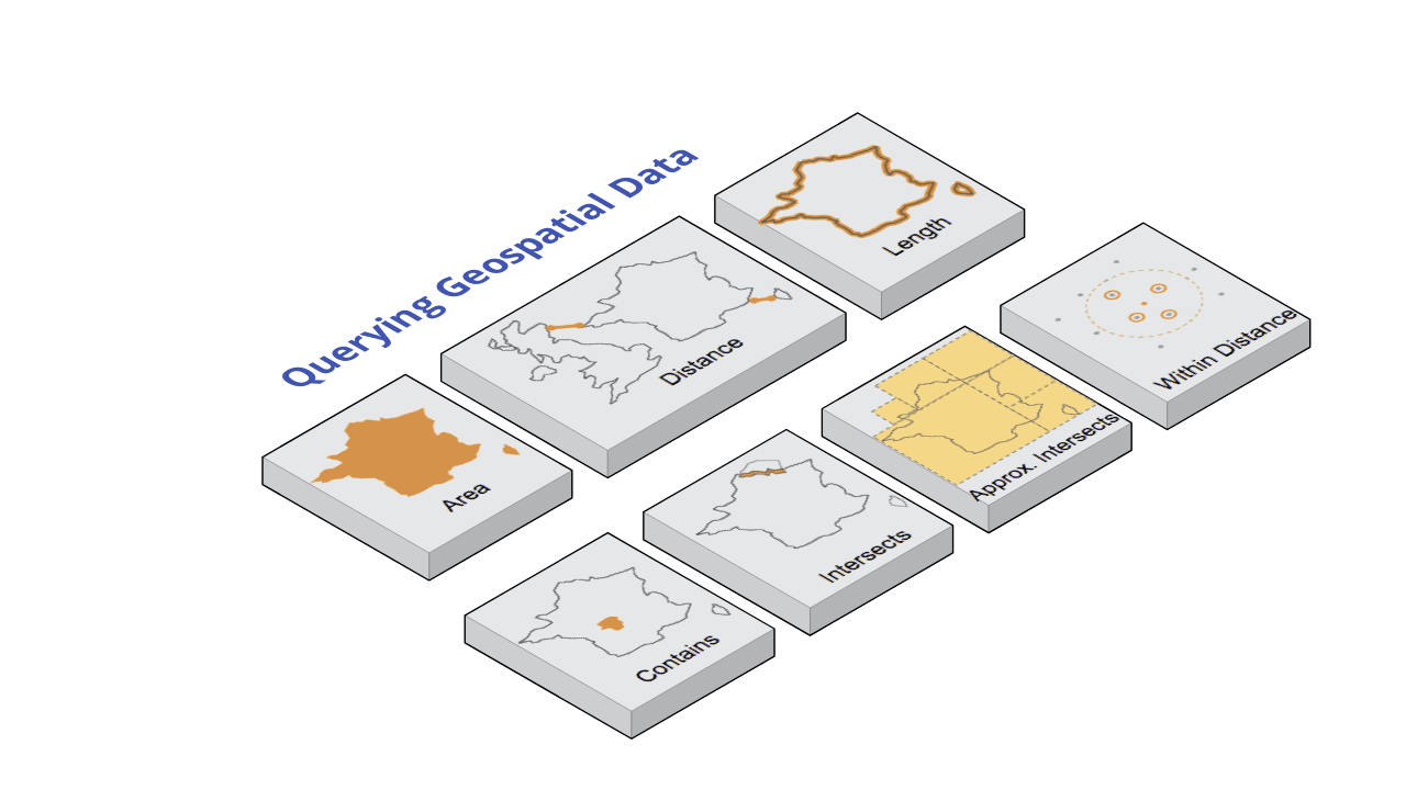
Area (GEOGRAPHY_AREA)
This measures the square meter area of a polygon.
We can find the area of a London borough in square meters. In this case, we are using Merton:
SELECT ROUND(GEOGRAPHY_AREA(geometry), 0) AS sqm
FROM london_boroughs
WHERE name = "Merton";
The output should be:
+---------------+
| sqm |
+---------------+
| 3.745656182E7 |
+---------------+
Since we also have hectares being stored for each borough, we can compare the result with the hectares, and the numbers are close. It is not a perfect match since the polygon data for the borough is storing a limited number of points, so the calculated area will be different. If we stored more data points, the accuracy would improve.
Distance (GEOGRAPHY_DISTANCE)
This measures the shortest distance between two geospatial objects, in meters. The function uses the standard metric for distance on a sphere.
We can find how far each London borough is from a particular borough. In this case, we are using Merton:
SELECT b.name AS neighbour, ROUND(GEOGRAPHY_DISTANCE(a.geometry, b.geometry), 0) AS distance_from_border
FROM london_boroughs a, london_boroughs b
WHERE a.name = "Merton"
ORDER BY distance_from_border
LIMIT 10;
The output should be:
+------------------------+----------------------+
| neighbour | distance_from_border |
+------------------------+----------------------+
| Lambeth | 0.0 |
| Kingston upon Thames | 0.0 |
| Merton | 0.0 |
| Wandsworth | 0.0 |
| Sutton | 0.0 |
| Croydon | 0.0 |
| Richmond upon Thames | 552.0 |
| Hammersmith and Fulham | 2609.0 |
| Bromley | 3263.0 |
| Southwark | 3276.0 |
+------------------------+----------------------+
Length (GEOGRAPHY_LENGTH)
This measures the length of a path. The path could also be the total perimeter of a polygon. Measurement is in meters.
Here we calculate the perimeter for London boroughs and order the result by the longest first.
SELECT name, ROUND(GEOGRAPHY_LENGTH(geometry), 0) AS perimeter
FROM london_boroughs
ORDER BY perimeter DESC
LIMIT 5;
The output should be:
+----------------------+-----------+
| name | perimeter |
+----------------------+-----------+
| Bromley | 76001.0 |
| Richmond upon Thames | 65102.0 |
| Hillingdon | 63756.0 |
| Havering | 63412.0 |
| Hounslow | 58861.0 |
+----------------------+-----------+
Contains (GEOGRAPHY_CONTAINS)
This determines if one object is entirely within another object.
In this example, we are trying to find all the London Underground stations within Merton:
SELECT b.name
FROM london_boroughs a, london_stations b
WHERE GEOGRAPHY_CONTAINS(a.geometry, b.geometry) AND a.name = "Merton"
ORDER BY name;
The output should be:
+-----------------+
|      name       |
+-----------------+
| Colliers Wood   |
| Morden          |
| South Wimbledon |
| Wimbledon       |
| Wimbledon Park  |
+-----------------+
Intersects (GEOGRAPHY_INTERSECTS)
This determines whether there is any overlap between two geospatial objects.
In this example, we are trying to determine which London borough Morden Station intersects:
SELECT a.name
FROM london_boroughs a, london_stations b
WHERE GEOGRAPHY_INTERSECTS(b.geometry, a.geometry) AND b.name = "Morden";
The output should be:
+--------+
| name |
+--------+
| Merton |
+--------+
Approx. Intersects (APPROX_GEOGRAPHY_INTERSECTS)
This is a fast approximation of the previous function.
SELECT a.name
FROM london_boroughs a, london_stations b
WHERE APPROX_GEOGRAPHY_INTERSECTS(b.geometry, a.geometry) AND b.name = "Morden";
The output should be:
+--------+
| name |
+--------+
| Merton |
+--------+
Within Distance (GEOGRAPHY_WITHIN_DISTANCE)
This determines whether two geospatial objects are within a certain distance of each other. Measurement is in meters.
In the following example, we try to find any London Underground stations within 100 meters of a centroid.
SELECT a.name
FROM london_stations a, london_boroughs b
WHERE GEOGRAPHY_WITHIN_DISTANCE(a.geometry, b.centroid, 100)
ORDER BY name;
The output should be:
+------------------------+
| name |
+------------------------+
| High Street Kensington |
+------------------------+
Visualization
Map of the London Underground
In our SingleStore database, we have stored geospatial data. We can use that data to create visualizations. To begin with, let's create a graph of the London Underground network.
We'll start by creating a new Databricks CE Python notebook. We'll call it Shortest Path. We'll attach our new notebook to our Spark cluster.
In a new code cell, let's add the following code to import several libraries:
import pandas as pd
import networkx as nx
import matplotlib.pyplot as plt
import folium
from folium import plugins
And now, we'll set up the connection to SingleStore:
%run ./Setup
In the next code cell we'll set some parameters for the SingleStore Spark Connector, as follows:
spark.conf.set("spark.datasource.singlestore.ddlEndpoint", cluster)spark.conf.set("spark.datasource.singlestore.user", "admin")spark.conf.set("spark.datasource.singlestore.password", password)spark.conf.set("spark.datasource.singlestore.disablePushdown", "false")We'll read the data from the three London Underground tables into Spark DataFrames and then convert them to Pandas:
df1 = (spark.read
.format("singlestore") .load("geo_db.london_connections"))
connections_df = df1.toPandas()
df2 = (spark.read
.format("singlestore") .load("geo_db.london_lines"))
lines_df = df2.toPandas()
df3 = (spark.read
.format("singlestore") .load("geo_db.london_stations"))
stations_df = df3.toPandas()
Next, we'll build a graph using NetworkX. The following code was inspired by an example on GitHub. The code creates nodes and edges to represent stations and the connections between them:
graph = nx.Graph()
for station_id, station in stations_df.iterrows():
graph.add_node(station["name"],
lon = station["longitude"],
lat = station["latitude"],
s_id = station["id"])
for connection_id, connection in connections_df.iterrows():
station1_name = stations_df.loc[stations_df["id"] == connection["station1"], "name"].item()
station2_name = stations_df.loc[stations_df["id"] == connection["station2"], "name"].item()
graph.add_edge(station1_name,
station2_name,
time = connection["time"],
line = connection["line"])
We can check the number of nodes and edges, as follows:
len(graph.nodes()), len(graph.edges())
The output should be:
(302, 349)
Next, we'll get the node positions. The following code was inspired by an example on DataCamp.
node_positions = {node[0]: (node[1]["lon"], node[1]["lat"]) for node in graph.nodes(data = True)}And we can check the values:
dict(list(node_positions.items())[0:5])
The output should be similar to:
{'Aldgate': (-0.0755, 51.5143),'All Saints': (-0.013, 51.5107),
'Alperton': (-0.2997, 51.5407),
'Angel': (-0.1058, 51.5322),
'Archway': (-0.1353, 51.5653)}
We'll now get the lines that connect stations:
edge_lines = [edge[2]["line"] for edge in graph.edges(data = True)]
And we can check the values:
edge_lines[0:5]
The output should be similar to:
[8, 3, 13, 13, 10]
From this information, we can find the line color:
edge_colours = [lines_df.loc[lines_df["line"] == line, "colour"].iloc[0] for line in edge_lines]
And we can check the values:
edge_colours[0:5]
The output should be similar to:
['#9B0056', '#FFD300', '#00A4A7', '#00A4A7', '#003688']
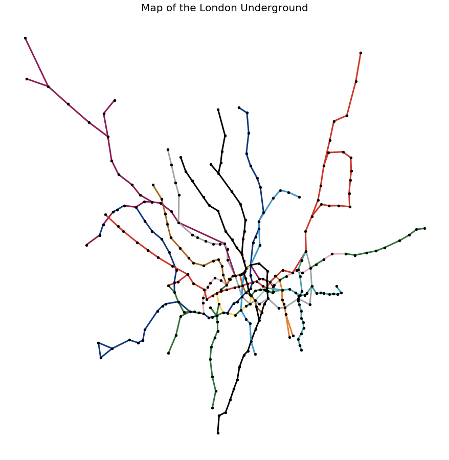
Now we can create a plot, as follows:
plt.figure(figsize = (12, 12))
nx.draw(graph,
pos = node_positions,
edge_color = edge_colours,
node_size = 20,
node_color = "black",
width = 3)
plt.title("Map of the London Underground", size = 20)plt.show()
This produces the image shown in Figure 9.
We can also represent the graph as a DataFrame. The following code was inspired by an example on GitHub.
network_df = pd.DataFrame()
lons, lats = map(nx.get_node_attributes, [graph, graph], ["lon", "lat"])
lines, times = map(nx.get_edge_attributes, [graph, graph], ["line", "time"])
for edge in list(graph.edges()):
network_df = network_df.append(
{"station_from" : edge[0],"lon_from" : lons.get(edge[0]),
"lat_from" : lats.get(edge[0]),
"station_to" : edge[1],
"lon_to" : lons.get(edge[1]),
"lat_to" : lats.get(edge[1]),
"line" : lines.get(edge),
"time" : times.get(edge)
}, ignore_index = True)
If we now merge this DataFrame with the London Underground lines, it gives us a complete picture of stations, coordinates, and lines between stations.
network_df = pd.merge(network_df, lines_df, how = "left", on = "line")
If we wish, this could now be stored back into SingleStore for future use. We can also visualize this using Folium, as follows:
London = [51.509865, -0.118092]
m = folium.Map(location = London, tiles = "Stamen Terrain", zoom_start = 12)
for i in range(0, len(stations_df)):
folium.Marker(
location = [stations_df.iloc[i]["latitude"], stations_df.iloc[i]["longitude"]],
popup = stations_df.iloc[i]["name"],
).add_to(m)
for i in range(0, len(network_df)):
folium.PolyLine(
locations = [(network_df.iloc[i]["lat_from"], network_df.iloc[i]["lon_from"]),
(network_df.iloc[i]["lat_to"], network_df.iloc[i]["lon_to"])],
color = network_df.iloc[i]["colour"],
weight = 3,
opacity = 1).add_to(m)
plugins.Fullscreen(
position = "topright",
title = "Fullscreen",
title_cancel = "Exit",
force_separate_button = True).add_to(m)
m
This produces a map, as shown in Figure 10. We can scroll and zoom the map. When clicked, a marker will show the station name, and the lines are colored according to the London Underground scheme.
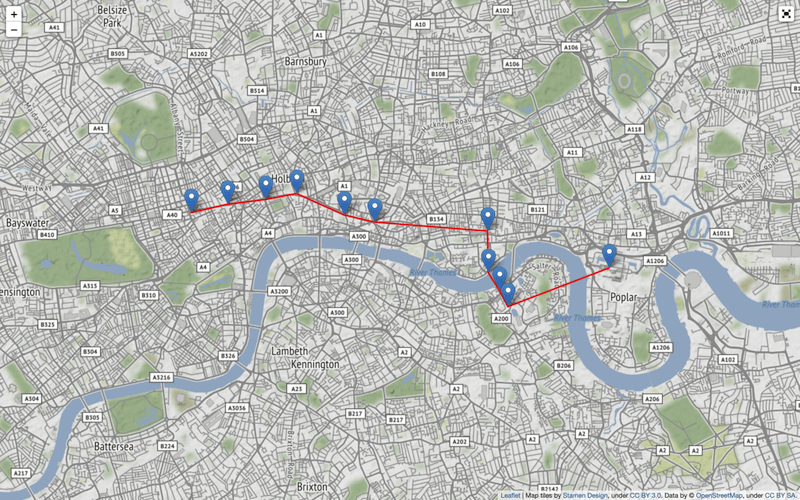
Shortest Path
We can also use the graph for more practical purposes. For example, by finding the shortest path between two stations.
We can use a built-in feature of NetworkX called shortest_path. Here we are looking to travel from Oxford Circus to Canary Wharf:
shortest_path = nx.shortest_path(graph, "Oxford Circus", "Canary Wharf", weight = "time")
We can check the route:
shortest_path
The output should be:
['Oxford Circus',
'Tottenham Court Road',
'Holborn',
'Chancery Lane',
"St. Paul's",
'Bank',
'Shadwell',
'Wapping',
'Rotherhithe',
'Canada Water',
'Canary Wharf']
To visualize the route, we can convert this to a DataFrame:
shortest_path_df = pd.DataFrame({"name" : shortest_path})And then merge it with the station's data so that we can get the geospatial data:
merged_df = pd.merge(shortest_path_df, stations_df, how = "left", on = "name")
We can now create a map using Folium, as follows:
m = folium.Map(tiles = "Stamen Terrain")
sw = merged_df[["latitude", "longitude"]].min().values.tolist()
ne = merged_df[["latitude", "longitude"]].max().values.tolist()
m.fit_bounds([sw, ne])
for i in range(0, len(merged_df)):
folium.Marker(
location = [merged_df.iloc[i]["latitude"], merged_df.iloc[i]["longitude"]],
popup = merged_df.iloc[i]["name"],
).add_to(m)
points = tuple(zip(merged_df.latitude, merged_df.longitude))
folium.PolyLine(points, color = "red", weight = 3, opacity = 1).add_to(m)
plugins.Fullscreen(
position = "topright",
title = "Fullscreen",
title_cancel = "Exit",
force_separate_button = True).add_to(m)
m
This produces a map, as shown in Figure 11. We can scroll and zoom the map. When clicked, a marker will show the station name.
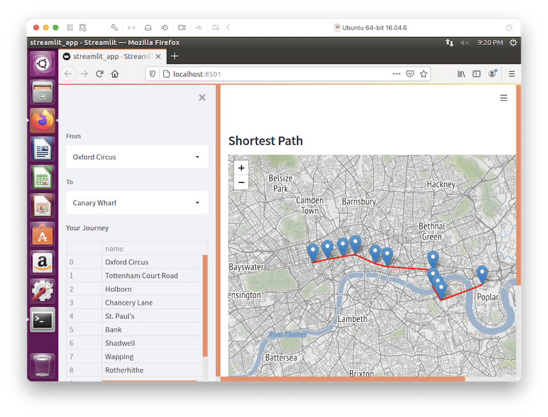
Bonus: Streamlit Visualization
We can use Streamlit to create a small application that allows us to select start and end stations for a journey on the London Underground, and the application will find the shotest path.
Install the Required Software
We need to install the following packages:
streamlit
streamlit-folium
pandas
networkx
folium
pymysql
These can be found in the requirements.txt file on GitHub. Run the file as follows:
pip install -r requirements.txt
Example Application
Here is the complete code listing for streamlit_app.py:
# streamlit_app.py
import streamlit as st
import pandas as pd
import networkx as nx
import folium
import pymysql
from streamlit_folium import folium_static
# Initialize connection.
def init_connection():
return pymysql.connect(**st.secrets["singlestore"])
conn = init_connection()
# Perform query.
connections_df = pd.read_sql("""SELECT *
FROM london_connections;
""", conn)
stations_df = pd.read_sql("""SELECT *
FROM london_stations
ORDER BY name;
""", conn)
stations_df.set_index("id", inplace = True)
st.subheader("Shortest Path")
from_name = st.sidebar.selectbox("From", stations_df["name"])to_name = st.sidebar.selectbox("To", stations_df["name"])
graph = nx.Graph()
for connection_id, connection in connections_df.iterrows():
station1_name = stations_df.loc[connection["station1"]]["name"]
station2_name = stations_df.loc[connection["station2"]]["name"]
graph.add_edge(station1_name, station2_name, time = connection["time"])
shortest_path = nx.shortest_path(graph, from_name, to_name, weight = "time")
shortest_path_df = pd.DataFrame({"name" : shortest_path})
merged_df = pd.merge(shortest_path_df, stations_df, how = "left", on = "name")
m = folium.Map(tiles = "Stamen Terrain")
sw = merged_df[["latitude", "longitude"]].min().values.tolist()
ne = merged_df[["latitude", "longitude"]].max().values.tolist()
m.fit_bounds([sw, ne])
for i in range(0, len(merged_df)):
folium.Marker(
location = [merged_df.iloc[i]["latitude"], merged_df.iloc[i]["longitude"]],
popup = merged_df.iloc[i]["name"],
).add_to(m)
points = tuple(zip(merged_df.latitude, merged_df.longitude))
folium.PolyLine(points, color = "red", weight = 3, opacity = 1).add_to(m)
folium_static(m)
st.sidebar.write("Your Journey", shortest_path_df)Create a Secrets File
Our local Streamlit application will read secrets from a file .streamlit/secrets.toml in our application's root directory. We need to create this file as follows:
# .streamlit/secrets.toml
[singlestore]
host = "<TO DO>"
port = 3306
database = "geo_db"
user = "admin"
password = "<TO DO>"
The <TO DO> for host and password should be replaced with the values obtained from the SingleStore Managed Service when creating a cluster.
Run the Code
We can run the Streamlit application as follows:
streamlit run streamlit_app.py
The output is a web browser that should look like Figure 12.
Feel free to experiment with the code to suit your needs.
Summary
In this article, we have seen a range of very powerful geospatial functions supported by SingleStore. Through examples, we have seen these functions working over our geospatial data. We have also seen how we can create graph structures and query those through various libraries. These libraries, combined with SingleStore, enable modeling and querying of graph structures with ease.
There are several improvements that we could make:
- The data on the London Underground needs to be updated. New stations and line extensions have been added to the network recently.
- We could also add additional transport modes, such as the London Tram Network.
- We could also add additional connection information about the transport network. For example, some stations may not be directly connected but may be within a short walking distance.
- Our visualization of the various Underground lines could also be improved since any route served by multiple lines only shows one of the lines.
- The shortest path is calculated on static data. It would be beneficial to extend our code to include real-time updates to the transport network to allow for delays.
Acknowledgments
This article would not have been possible without the examples provided by other authors and developers.
There is a wonderful quote attributed to Sir Isaac Newton:
If I have seen further it is by standing on the shoulders of giants.
Recommend
About Joyk
Aggregate valuable and interesting links.
Joyk means Joy of geeK