This article implements Passing-Bablok regression in SAS. Passing-Bablok regression is a one-variable regression technique that is used to compare measurements from different instruments or medical devices. The measurements of the two variables (X and Y) are both measured with errors. Consequently, you cannot use ordinary linear regression, which assumes that one variable (X) is measured without error. Passing-Bablok regression is a robust nonparametric regression method that does not make assumptions about the distribution of the expected values or the error terms in the model. It also does not assume that the errors are homoskedastic.

Several readers have asked about Passing-Bablok regression because I wrote an article about Deming regression, which is similar. On the SAS Support Communities, there was a lively discussion in response to a program by KSharp in which he shows how to use Base SAS procedures to perform a Passing-Bablok regression. In response to this interest, this article shares a SAS/IML program that performs Passing-Bablok regression.

An overview of Passing-Bablok regression

Passing-Bablok regression (Passing and Bablok, 1983, J. Clin. Chem. Clin. Biochem., henceforth denote PB) fits a line through X and Y measurements. The X and Y variables measure the same quantity in the same units. Usually, X is the "gold standard" technique, whereas Y is a new method that is cheaper, more accurate, less invasive, or has some other favorable attributes. Whereas Deming regression assumes normal errors, Passing-Bablok regression can handle any error distribution provided that the measurement errors for both methods follow the same distribution. Also, the variance of each method does not need to be constant across the range of data. All that is required is that the ratio of the variances is constant. The Passing-Bablok method is robust to outliers in X or Y.

Assume you have N pairs of observations {(xi, yi), i=1..N}, where X and Y are different ways to measure the same quantity. Passing-Bablok regression determines whether the measurements methods are equivalent by estimating a line y = a + b*x. The estimate of the slope (b) is based on the median of pairs of slopes Sij = (yi - yj) / (xi - xj) for i < j. You must be careful when xi=xj. PB suggest assigning a large positive value when xi=xj and yi > yj and a large negative value when xi=xj and yi < yj. If xi=xj and yi=yj, the difference is not computed or used.

The Passing-Bablok method estimates the regression line y = a + b*x by using the following steps:

1. Compute all the pairwise slopes. For vertical slopes, use large positive or negative values, as appropriate.
2. Exclude slopes that are exactly -1. The reason is technical, but it involves ensuring the same conclusions whether you regress Y onto X or X onto Y.
3. Ideally, we would estimate the slope of the regression line (b) as the median of all the pairwise slopes of the points (xi, yi) and (xj, yj), where i < j. This is a robust statistic and is similar to Theil-Sen regression. However, the slopes are not independent, so the median can be a biased estimator. Instead, estimate the slope as the shifted median of the pairwise slopes.
4. Estimate the intercept, a, as the median of the values {yi – bxi}.
5. Use a combination of symmetry, rank-order statistics, and asymptotics to obtain confidence intervals (CIs) for b and a.
6. You can use the confidence intervals (CIs) to assess whether the two methods are equivalent. In terms of the regression estimates, the CI for the intercept (a) must contain 0 and the CI for the slope (b) must contain 1. This article uses only the CIs proposed by Passing and Bablok. Some software support jackknife or bootstrap CIs, but it is sometimes a bad idea to use resampling methods to estimate the CI of a median, so I do not recommend bootstrap CIs for Passing-Bablok regression.

Implement Passing-Bablok regression in SAS

Because the Passing-Bablok method relies on computing vectors and medians, the SAS/IML language is a natural language for implementing the algorithm. The implementation uses several helper functions from previous articles:

The following modules implement the Passing-Bablok algorithm in SAS and store the modules for future use:

%let INFTY = 1E12;         /* define a big number to use as "infinity" for vertical slopes */
proc iml;
/* Extract only the values X[i,j] where i < j.
   https://blogs.sas.com/content/iml/2012/08/16/extract-the-lower-triangular-elements-of-a-matrix.html */
   start StrictLowerTriangular(X);
   v = cusum( 1 || (ncol(X):2) );
   return( remove(vech(X), v) );
finish;
/* Compute pairwise differences:
   https://blogs.sas.com/content/iml/2011/02/09/computing-pairwise-differences-efficiently-of-course.html */ 
start PairwiseDiff(x);   /* x is a column vector */
   n = nrow(x);   
   m = shape(x, n, n);   /* duplicate data */
   diff = m` - m;        /* pairwise differences */
   return( StrictLowerTriangular(diff) );
finish;
 
/* Implement the Passing-Bablok (1983) regression method */
start PassingBablok(_x, _y, alpha=0.05, debug=0);
   keepIdx = loc(_x^=. & _y^=.);      /* 1. remove missing values */
   x = _x[keepIdx]; y = _y[keepIdx];
   nObs = nrow(x);                    /* sample size of nonmissing values */
 
   /* 1. Compute all the pairwise slopes. For vertical, use large positive or negative values. */
   DX = T(PairwiseDiff(x));           /* x[i] - x[j] */
   DY = T(PairwiseDiff(y));           /* y[i] - y[j] */
 
   /* "Identical pairs of measurements with x_i=x_j and y_i=y_j
      do not contribute to the estimation of beta." (PB, p 711) */
   idx = loc(DX^=0 | DY^=0);          /* exclude 0/0 slopes (DX=0 and DY=0) */
   G = DX[idx] || DY[idx] || j(ncol(idx), 1, .); /* last col is DY/DX */
   idx = loc( G[,1] ^= 0 );           /* find where DX ^= 0 */
   G[idx,3] = G[idx,2] / G[idx,1];    /* form Sij = DY / DX for DX^=0 */
 
   /* Special cases:
      1) x_i=x_j, but y_i^=y_j   ==> Sij = +/- infinity
      2) x_i^=x_j, but y_i=y_j   ==> Sij = 0
      "The occurrence of any of these special cases has a probability 
      of zero (experimental data should exhibit these cases very rarely)."
 
      Passing and Bablok do not specify how to handle, but one way is
      to keep these values within the set of valid slopes. Use large 
      positive or negative numbers for +infty and -infty, respectively.
   */
   posIdx = loc(G[,1]=0 & G[,2]>0);    /* DX=0 & DY>0 */
   if ncol(posIdx) then G[posIdx,3] =  &INFTY;
   negIdx = loc(G[,1]=0 & G[,2]<0);    /* DX=0 & DY<0 */
   if ncol(negIdx) then G[negIdx,3] = -&INFTY;
   if debug then PRINT (T(1:nrow(G)) || G)[c={"N" "DX" "DY" "S"}];
 
   /* 2. Exclude slopes that are exactly -1 */
   /* We want to be able to interchange the X and Y variables. 
      "For reasons of symmetry, any Sij with a value of -1 is also discarded." */
   idx = loc(G[,3] ^= -1); 
   S = G[idx,3];
   N = nrow(S);                      /* number of valid slopes */
   call sort(S);                     /* sort slopes ==> pctl computations easier */
   if debug then print (S`)[L='sort(S)'];
 
   /* 3. Estimate the slope as the shifted median of the pairwise slopes. */
   K = sum(S < -1);                  /* shift median by K values */
   b = choose(mod(N,2),              /* estimate of slope */
              S[(N+1)/2+K ],         /* if N odd, shifted median */
              mean(S[N/2+K+{0,1}])); /* if N even, average of adjacent values */
   /* 4. Estimate the intercept as the median of the values {yi – bxi}. */
   a = median(y - b*x);              /* estimate of the intercept, a */
 
   /* 5. Estimate confidence intervals. */
   C = quantile("Normal", 1-alpha/2) * sqrt(nObs*(nObs-1)*(2*nObs+5)/18);
   M1 = round((N - C)/2);
   M2 = N - M1 + 1;
   if debug then PRINT K C M1 M2 (M1+K)[L="M1+K"] (M2+k)[L="M1+K"];
   CI_b = {. .};                     /* initialize CI to missing */
   if 1 <= M1+K & M1+K <= N then CI_b[1] = S[M1+K];
   if 1 <= M2+K & M2+K <= N then CI_b[2] = S[M2+K];
   CI_a = median(y - CI_b[,2:1]@x);  /* aL=med(y-bU*x); aU=med(y-bL*x); */
 
   /* return a list that contains the results */
   outList = [#'a'=a, #'b'=b, #'CI_a'=CI_a, #'CI_b'=CI_b]; /* pack into list */
   return( outList );
finish;
 
store module=(StrictLowerTriangular PairwiseDiff PassingBablok);
quit;

Notice that the PassingBablok function returns a list. A list is a convenient way to return multiple statistics from a function.

Perform Passing-Bablok regression in SAS

Having saved the SAS/IML modules, let's see how to call the PassingBablok routine and analyze the results. The following DATA step defines 102 pairs of observations. These data were posted to the SAS Support Communities by @soulmate. To support running regressions on multiple data sets, I use macro variables to store the name of the data set and the variable names.

data PBData;
label x="Method 1" y="Method 2";
input x y @@;
datalines;
0.07 0.07  0.04 0.10  0.07 0.08  0.05 0.10  0.06 0.08
0.06 0.07  0.03 0.05  0.04 0.05  0.05 0.08  0.05 0.10
0.12 0.21  0.10 0.17  0.03 0.11  0.18 0.24  0.29 0.33
0.05 0.05  0.04 0.05  0.11 0.21  0.38 0.36  0.04 0.05
0.03 0.06  0.06 0.07  0.46 0.27  0.08 0.05  0.02 0.09
0.12 0.23  0.16 0.25  0.07 0.10  0.07 0.07  0.04 0.06
0.11 0.23  0.23 0.21  0.15 0.20  0.05 0.07  0.04 0.14
0.05 0.11  0.17 0.26  8.43 8.12  1.86 1.47  0.17 0.27
8.29 7.71  5.98 5.26  0.57 0.43  0.07 0.10  0.06 0.11
0.21 0.24  8.29 7.84  0.28 0.23  8.25 7.79  0.18 0.25
0.17 0.22  0.15 0.21  8.33 7.67  5.58 5.05  0.09 0.14
1.00 3.72  0.09 0.13  3.88 3.54  0.51 0.42  4.09 3.64
0.89 0.71  5.61 5.18  4.52 4.15  0.09 0.12  0.05 0.05
0.05 0.05  0.04 0.07  0.05 0.07  0.09 0.11  0.03 0.05
2.27 2.08  1.50 1.21  5.05 4.46  0.22 0.25  2.13 1.93
0.05 0.08  4.09 3.61  1.46 1.13  1.20 0.97  0.02 0.05
1.00 1.00  3.39 3.11  1.00 0.05  2.07 1.83  6.68 6.06
3.00 2.97  0.06 0.09  7.17 6.55  1.00 1.00  2.00 0.05
2.91 2.45  3.92 3.36  1.00 1.00  7.20 6.88  6.42 5.83
2.38 2.04  1.97 1.76  4.72 4.37  1.64 1.25  5.48 4.77
5.54 5.16  0.02 0.06
;
 
%let DSName = PBData;    /* name of data set */
%let XVar = x;           /* name of X variable (Method 1) */
%let YVar = y;           /* name of Y variable (Method 2) */
 
title "Measurements from Two Methods";
proc sgplot data=&DSName;
   scatter x=&XVar y=&YVar;
   lineparm x=0 y=0 slope=1 / clip;    /* identity line: Intercept=0, Slope=1 */
   xaxis grid;
   yaxis grid;
run;

The graph indicates that the two measurements are linearly related and strongly correlated. It looks like Method 1 (X) produces higher measurements than Method 2 (Y) because most points are to the right of the identity line. Three outliers are visible. The Passing-Bablok regression should be robust to these outliers.

The following SAS/IML program analyzes the data by calling the PassingBablok function:

proc iml;
load module=(StrictLowerTriangular PairwiseDiff PassingBablok);
use &DSName; 
   read all var {"&XVar"} into x;
   read all var {"&YVar"} into y;
close;
 
R = PassingBablok(x, y);
ParameterEstimates = (R$'a' || R$'CI_a') //        /* create table from the list items */
                     (R$'b' || R$'CI_b');
print ParameterEstimates[c={'Estimate' 'LCL' 'UCL'} r={'Intercept' 'Slope'}];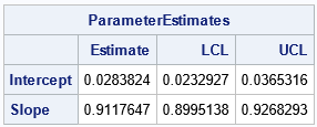

The program reads the X and Y variables and calls the PassingBablok function, which returns a list of statistics. You can use the ListPrint subroutine to print the items in the list, or you can extract the items and put them into a matrix, as in the example.

The output shows that the Passing-Bablok regression line is Y = 0.028 + 0.912*X. The confidence interval for the slope parameter (b) does NOT include 1, which means that we reject the null hypothesis that the measurements are related by a line that has unit slope. Even if the CI for the slope had contained 1, the CI for the Intercept (a) does not include 0. For these data, we reject the hypothesis that the measurements from the two methods are equivalent.

Of course, you could encapsulate the program into a SAS macro that performs Passing-Bablok regression.

A second example of Passing-Bablok regression in SAS

For completeness, the following example shows results for two methods that are equivalent. The output shows that the CI for the slope includes 1 and the CI for the intercept includes 0:

%let DSName = PBData2;    /* name of data set */
%let XVar = m1;           /* name of X variable (Method 1) */
%let YVar = m2;           /* name of Y variable (Method 2) */
 
data &DSName;
label x="Method 1" y="Method 2";
input m1 m2 @@;
datalines;
10.1 10.1  10.5 10.6  12.8 13.1   8.7  8.7  10.8 11.5 
10.6 10.4   9.6  9.9  11.3 11.3   7.7  7.5  11.5 11.9 
 7.9  7.8   9.9  9.7   9.3  9.9  16.3 16.2   9.4  9.8 
11.0 11.8   9.1  8.7  12.2 11.9  13.4 12.6   9.2  9.5 
 8.8  9.1   9.3  9.2   8.5  8.7   9.6  9.7  13.5 13.1 
 9.4  9.1   9.5  9.6  10.8 11.3  14.6 14.8   9.7  9.3 
16.4 16.5   8.1  8.6   8.3  8.1   9.5  9.6  20.3 20.4 
 8.6  8.5   9.1  8.8   8.8  8.7   9.2  9.9   8.1  8.1 
 9.2  9.0  17.0 17.0  10.2 10.0  10.0  9.8   6.5  6.6 
 7.9  7.6  11.3 10.7  14.2 14.1  11.9 12.7   9.9  9.4 
;
 
proc iml;
load module=(StrictLowerTriangular PairwiseDiff PassingBablok);
use &DSName; 
   read all var {"&XVar"} into x;
   read all var {"&YVar"} into y;
close;
 
R = PassingBablok(x, y);
ParameterEstimates = (R$'a' || R$'CI_a') // 
                     (R$'b' || R$'CI_b');
print ParameterEstimates[c={'Estimate' 'LCL' 'UCL'} r={'Intercept' 'Slope'}];
QUIT;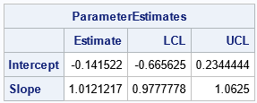

For these data, the Passing-Bablok regression line is Y = 0.028 + 0.912*X. The confidence interval for the Slope term is [0.98, 1.06], which contains 1. The confidence interval for the Intercept is [-0.67, 0.23], which contains 0. Thus, these data suggest that the two methods are equivalent ways to measure the same quantity.

Summary

This article shows how to implement Passing-Bablok regression in SAS by using the SAS/IML language. It also explains how Passing-Bablok regression works and why different software might provide different confidence intervals. You can download the complete SAS program that implements Passing-Bablok regression and creates the graphs and tables in this article.

Further Reading

• "An example of Passing-Bablok Regression in SAS" by KSharp is a program that uses only Base SAS procedures. He also includes a PDF of the Passing-Bablok paper.
• "Passing-Bablok Regression: R code for SAS users" by Clint Stevenson. Includes a discussion of why the default regression in the mcr package in R is different from method in the Passing-Bablok paper.
• Documentation of the Passing-Bablok regression in the NCSS software package.
• The mcr package in R by Manuilova, Schuetzenmeister, and Model contains several regression methods for method-comparison regression.

Appendix: Comparing the results of Passing-Bablok regression

The PB paper is slightly ambiguous about how to handle certain special situations in the data. The ambiguity is in the calculation of confidence intervals. Consequently, if you run the same data through different software, you are likely to obtain the same point estimates, but the confidence intervals might be slightly different (maybe in the third or fourth decimal place), especially when there are repeated X values that have multiple Y values. For example, I have compared my implementation to MedCalc software and to the mcr package in R. The authors of the mcr package made some choices that are different from the PB paper. By looking at the code, I can see that they handle tied data values differently from the way I handle them.