I was inspired to write this post based on an article written by my colleague. I will build on that article by introducing Jupyter Notebook to the mix. This is the next installment in the series of tutorials on CockroachDB and Docker Compose.

You can find the older posts here: Part 1, Part 2, Part 3, Part 4, Part 5.

• Information on CockroachDB can be found here.
• Information on the Jupyter Notebook project can be found here.
• Information on the R language can be found here.
• Information on the RPostgres driver can be found here.

We're going to continue using our trusty docker-compose. Jupyter project publishes its images on Docker Hub. This time, we're going to use a slightly different image than the one from the previous post. Whereas we've used a minimal image last time, we need to use image: jupyter/r-notebook this time around that includes an R kernel. So the line we're going to replace is image: jupyter/minimal-notebook. Also, make sure to update the cockroach image to the latest. My diff on the previous docker-compose is below:

6c6
<    image: cockroachdb/cockroach:v19.2.4
---
>    image: cockroachdb/cockroach:v19.2.3
16c16
<    image: jupyter/r-notebook
---
>    image: jupyter/minimal-notebook

1. Install prerequisites for R.

Jupyter notebook for R ships with many packages to get started with R but since we're working with a Postgresql compliant database, we need some additional libraries. All of the Jupyter images I've worked with are shipped with tight security. The notebook is accessible via a token and sudo is not enabled by default. For that reason, we have to rely on the logs to get the notebook url and access the notebook container by passing --user root.

docker exec -it --user root jupyter bash

This will allow us to install some of the OS packages we need to complete this tutorial. We need a package called RPostgres and we will be able to fetch it from the Cran repo once we installed libpq-dev OS package.

After executing the previous command, we should be inside the container with the root login. Update the base OS repo and install the package.

root@7cc6323da05b:~# apt-get update && apt-get install libpq-dev

1. Initialize a CockroachDB workload.

To make things a bit more interesting, we're going to generate some synthetic data for us to work with. CRDB comes with a workload utility to make this step much easier. Read more here.

docker exec -it crdb-1 ./cockroach workload init movr

I200224 15:53:39.998976 1 workload/workloadsql/dataload.go:135  imported users (0s, 50 rows)
I200224 15:53:40.007592 1 workload/workloadsql/dataload.go:135  imported vehicles (0s, 15 rows)
I200224 15:53:40.038055 1 workload/workloadsql/dataload.go:135  imported rides (0s, 500 rows)
I200224 15:53:40.066728 1 workload/workloadsql/dataload.go:135  imported vehicle_location_histories (0s, 1000 rows)
I200224 15:53:40.093848 1 workload/workloadsql/dataload.go:135  imported promo_codes (0s, 1000 rows)

We are now ready to start exploring CockroachDB with R inside the Jupyter notebook.

1. Open Jupyter notebook.

If you've followed the previous posts, you can find the url to the notebook with the command docker logs jupyter. Simply copy the url and paste it into a browser window.

[C 15:36:12.727 NotebookApp]

    To access the notebook, open this file in a browser:
        file:///home/jovyan/.local/share/jupyter/runtime/nbserver-7-open.html
    Or copy and paste one of these URLs:
        http://88dee83ff5d0:8888/?token=33df2a270b9e58774bc79b6d8c3184b76aecf82b457b5043
     or http://127.0.0.1:8888/?token=33df2a270b9e58774bc79b6d8c3184b76aecf82b457b5043

1. Install the necessary R libraries.

install.packages('devtools', repos = 'http://cran.us.r-project.org')
install.packages('ggplot2', repos = 'http://cran.us.r-project.org')
install.packages('dplyr', repos = 'http://cran.us.r-project.org')
install.packages("dbplyr", repos = "https://cloud.r-project.org")
install.packages('RPostgres', repos = 'http://cran.us.r-project.org')

This step will take a few minutes and unfortunately, there is no interactive way to know the progress unless you tail the logs of the container.

docker logs jupyter -f

This will tailor 'f' for 'follow' the logs produced by the Jupyter container.

Depending on the environment, RPostgres package may or may not fail, in this situation, we installed libpq-dev and that was sufficient. Other times, we may need to install RPostgres using a different approach. Here's a snippet of code, I'd used elsewhere:

# Workaround
install.packages("remotes")
# will prompt for additional packages to be upgraded, ignoring..
remotes::install_github("r-dbi/RPostgres", upgrade = c("never"))

R allows installation of packages from remote repositories like Github, BitBucket, etc. Here, I fetch the dev build of the RPostgres driver from their Github. I'm also passing a flag to ignore any of the prompts to upgrade existing libraries.

1. Explore CRDB with R!

Enter the following R code into the Jupyter cell and execute:

require("ggplot2")
library(DBI)
# Connect to the default CockroachDB instance and MovR database
con <- dbConnect(RPostgres::Postgres(),dbname = "movr",
                 host = "crdb-1", port = 26257,
                 user = "root")
df_users_64 <- dbGetQuery(con, "select city, count(*) from users group by city;")
str(df_users_64)

Based on the code comment, you may be able to tell that we're connecting to a database instance on host crdb-1 with port 26257 and user root. We're also executing a standard SQL query and saving the output of which in a dataframe. Then we're casting the dataframe as a string to view the output.

'data.frame':   9 obs. of  2 variables:
 $ city : chr  "amsterdam" "boston" "los angeles" "new york" ...
 $ count:integer64 5 6 6 6 6 5 5 6 ...

Here's the same result using cockroach SQL shell:

root@:26257/movr> select city, count(*) from users group by city;
      city      | count
+---------------+-------+
  amsterdam     |     5
  boston        |     6
  los angeles   |     6
  new york      |     6
  paris         |     6
  rome          |     5
  san francisco |     5
  seattle       |     6
  washington dc |     5
(9 rows)

Time: 1.8026ms

You may notice that some of the output is truncated:

 $ count:integer64 5 6 6 6 6 5 5 6 ...

We need to cast the count to a different precision, something the inspiration article above talks about. We're going to use int4 cast in our SQL query.

select city, count(*)::int4 from users group by city;

root@:26257/movr> select city, count(*)::int4 from users group by city;
      city      | count
+---------------+-------+
  amsterdam     |     5
  boston        |     6
  los angeles   |     6
  new york      |     6
  paris         |     6
  rome          |     5
  san francisco |     5
  seattle       |     6
  washington dc |     5
(9 rows)

Time: 2.1037ms

Same result but a more accurate precision.

'data.frame':   9 obs. of  2 variables:
 $ city : chr  "amsterdam" "boston" "los angeles" "new york" ...
 $ count: int  5 6 6 6 6 5 5 6 5

This step is necessary as ggplot will throw out a warning. Again, something the inspiration article mentions.

1. Plot the results.

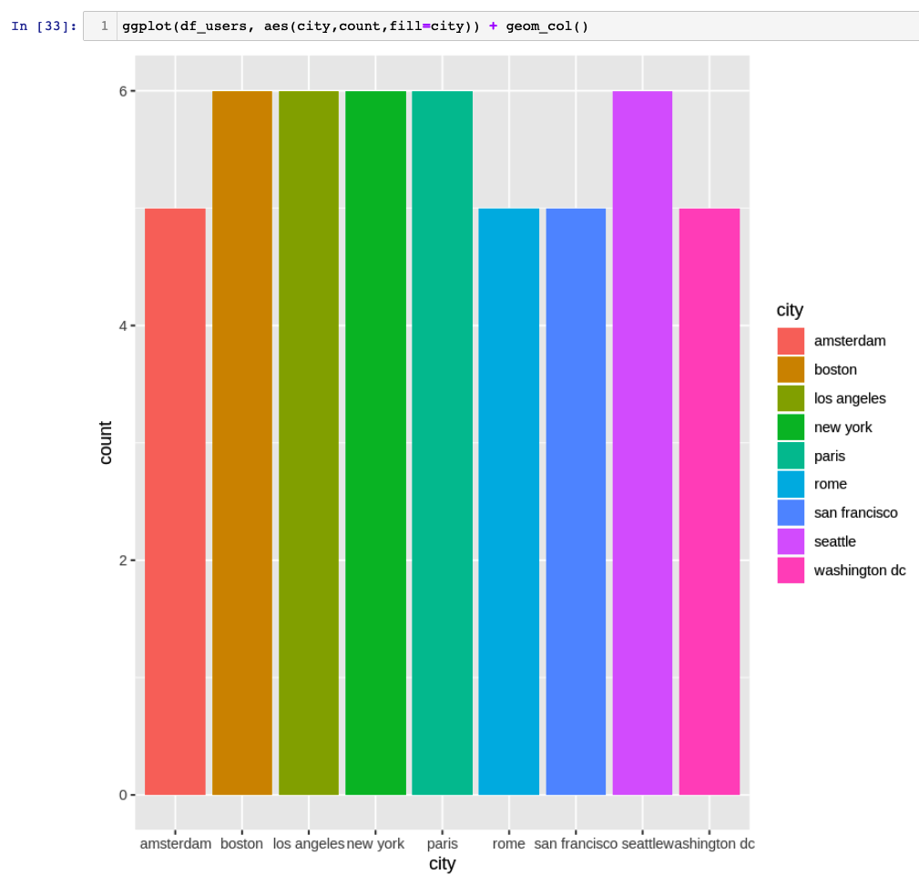
Now we can pass the data frame to ggplot utility and plot the graph of users per city.

ggplot(df_users, aes(city,count,fill=city)) + geom_col()

1. Explore vehicles table.

Movr database comes with several tables for a ride-sharing application. Let's look at the available vehicle types.

root@:26257/movr> select type, count(*) from vehicles group by type;
     type    | count
+------------+-------+
  scooter    |     7
  skateboard |     6
  bike       |     2
(3 rows)

Time: 1.6258ms

Back in the Jupyter Notebook:

df_vehicles <- dbGetQuery(con, "select type, count(*) from vehicles group by type;")
str(df_vehicles)

'data.frame':   3 obs. of  2 variables:
 $ type : chr  "skateboard" "bike" "scooter"
 $ count: int  6 2 7

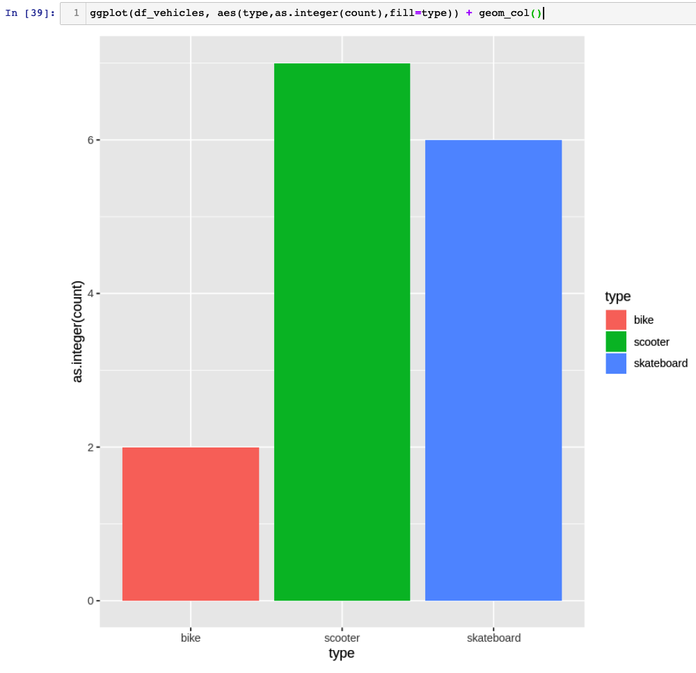
1. Graph this dataframe.

This time, we're using the other workaround from Robert's article and casting type count as as.integer(count) into ggplot.

ggplot(df_vehicles, aes(type,as.integer(count),fill=type)) + geom_col()

1. Explore additional RPostgres functionality.

# list tables
dbListTables(con)

# write to a table
dbWriteTable(con, "mtcars", mtcars)
dbListTables(con)

# list columns in a table
dbListFields(con, "rides")

# read from a table
dbReadTable(con, "rides")

# instead of casting dataframe as a string, we can use built-in functionality to fetch the results
res <- dbSendQuery(con, "SELECT city, count(*) FROM rides GROUP BY city;")
dbFetch(res)

# clear the results variable
dbClearResult(res)

# chunk results at a time
res <- dbSendQuery(con, "SELECT city, count(*) FROM rides GROUP BY city;")
while(!dbHasCompleted(res)){
  chunk <- dbFetch(res, n = 5)
  print(nrow(chunk))
}

# clear the result
dbClearResult(res)

# finally, disconnect from the database
dbDisconnect(con)

I hope you've enjoyed this tutorial and will come back soon for more. Please share your feedback in the comments.